https://ift.tt/3Erj9mC Manufacturing strikes in the United States plotted against time (Data source: R data sets ) (Image by Author) A s...
A step-by-step tutorial to get up and running with the Poisson HMM
A Poisson Hidden Markov Model is a mixture of two regression models: A Poisson regression model which is visible and a Markov model which is ‘hidden’. In a Poisson HMM, the mean value predicted by the Poisson model depends on not only the regression variables of the Poisson model, but also on the current state or regime that the hidden Markov process is in.
In an earlier article, we looked at the architecture of the Poisson Hidden Markov Model and we inspected its theoretical underpinnings. If you are new to Markov Models or the Poisson HMM, I will encourage you to review it here:
The Poisson Hidden Markov Model for Time Series Regression
In this article, we will go walk through a step by step tutorial in Python and statsmodels for building and training a Poisson HMM on the real world data set of labor strikes in US manufacturing that is used extensively in the literature on statistical modeling.
The MANUFACTURING STRIKES data set
To illustrate the model fitting procedure, we will use the following open source data set:
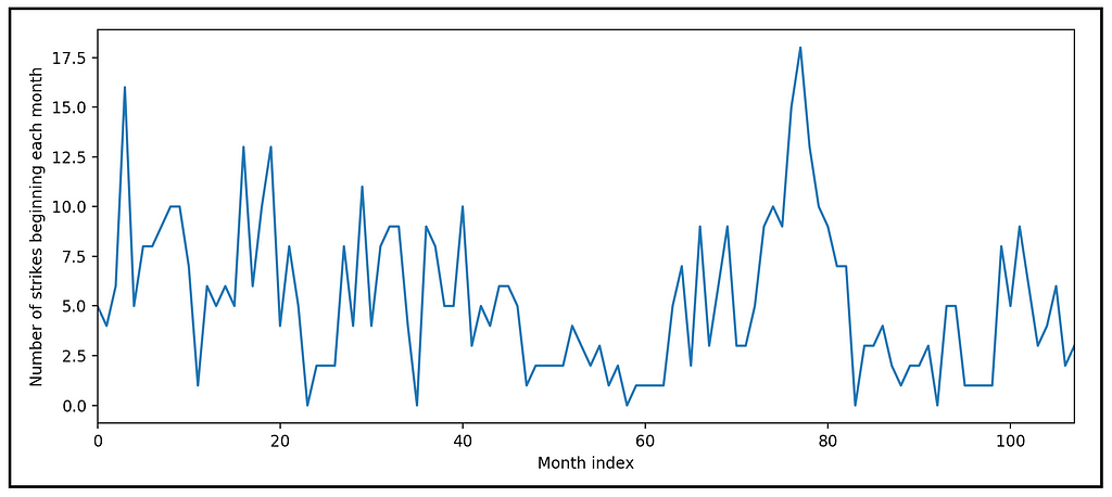
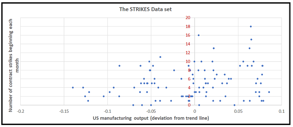
The data set is a monthly time series showing the relationship between U.S. manufacturing activity measured as a departure from the trend line, and the number of contract strikes in U.S. manufacturing industries beginning each month from 1968 through 1976.
This data set is available in R and it can be fetched using the Python statsmodels Datasets package.
The tutorial in this article uses Python, not R.
Regression goal
Our goal is to investigate the effect of manufacturing output (the output variable) on the incidence of manufacturing strikes (the strikes variable). In other words, does the variance in manufacturing output ‘explain’ the variance in the number of monthly strikes?
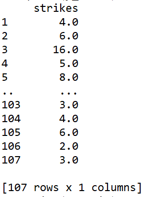
Let’s import all the required packages, load the strikes data set into a Pandas DaraFrame, and inspect a plot of strikes against time:
import math
import numpy as np
import statsmodels.api as sm
from statsmodels.base.model import GenericLikelihoodModel
from scipy.stats import poisson
from patsy import dmatrices
import statsmodels.graphics.tsaplots as tsa
from matplotlib import pyplot as plt
from statsmodels.tools.numdiff import approx_hess1, approx_hess2, approx_hess3
#Download the data set and load it into a Pandas Dataframe
strikes_dataset = sm.datasets.get_rdataset(dataname='StrikeNb', package='Ecdat')
#Plot the number of strikes starting each month
plt.xlabel('Month index')
plt.ylabel('Number of strikes beginning each month')
strikes_data['strikes'].plot()
plt.show()
We see the following plot:
The up-down whipsaw pattern of strikes suggests that the time series may be auto-correlated. Let’s verify this by looking at the auto-correlation plot of the strikes column:
tsa.plot_acf(strikes_data['strikes'], alpha=0.05)
plt.show()
We see the following plot:
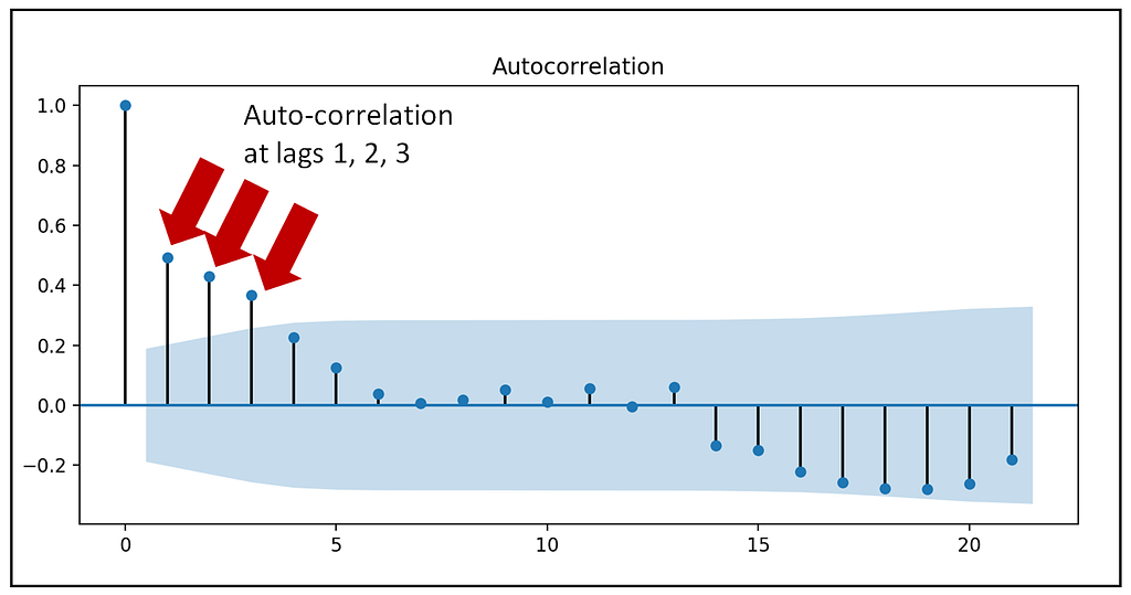
The perfect correlation at lag 0 is to be ignored as a value is always perfectly correlated with itself. There is a strong correlation at lag-1. The correlations at lags 2 and 3 are likely to be a domino effect of the correlation at lag 1. This can be confirmed by plotting the partial auto-correlation plot of strikes.
tsa.plot_pacf(strikes_data['strikes'], alpha=0.05)
plt.show()
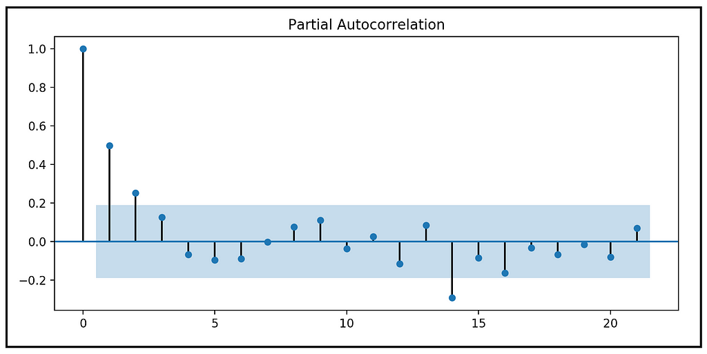
The partial auto-correlation plot reveals the following:
- The partial auto-correlation is 1.0 at LAG-0. This is expected, and to be ignored.
- The PACF plot shows a strong partial auto-correlation at LAG-1, which suggests an AR(1) process.
- The correlation at LAG-2 is just outside the 5% significance bounds. So, it may or may not be significant.
On the whole, the ACF and PACF plots indicate a definite, and strong auto-regressive influence at LAG-1. Hence, in addition to the output variable, we should include the lagged version of strikes at LAG-1 as a regression variable.
Regression strategy
Our strategy will be based upon regressing strikes on both output and on the time-lagged copy of strikes at lag-1.
Since strikes contains whole numbered data, we will use a Poisson regression model to study the relationship between output and strikes.
We will additional hypothesize that the manufacturing strikes data cycles between periods of low and high variability which can be modeled using a 2-state discrete Markov process.
Why did we choose only 2 regimes for the Markov model? Why not 3 or 4 regimes? The answer is simply that it is best to start with a Markov model with the least possible states so as to avoid over-fitting.
In summary, we will use a 2-state Poisson Hidden Markov Model to study the relationship of manufacturing output on strikes.
Therefore, we have:
Dependent variable (endogenous variable)
y = strikes
Regression variables (exogenous variables)
X = [output, strikes_LAG_1] + Hidden Markov model related variables which we will soon describe.
We’ll first spec-out the Poisson portion of the model, and then see how to ‘mix-in’ the Markov model.
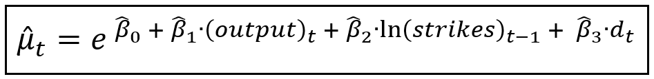
The Poisson model’s mean (without considering the effect of the Markov model) can be expressed as follows:

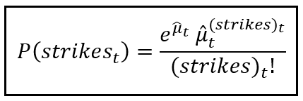
Since we are assuming that strikes is Poisson distributed, it’s Probability Mass Function is as follows:
Dealing with ‘model explosion’ and zero valued data
Our Poisson model has a problem. Let’s take a look at the specification of the mean again:
If the coefficient β_2 of the (strikes)_(t-1) term turns out to be greater than 0, we will face what is colorfully called the ‘model explosion’ effect, caused by a positive feedback loop from (strikes)_(t-1) to (strikes)_t. The solution is to replace (strikes)_(t-1) with its natural logarithm ln (strikes)_(t-1). But (strikes)_(t-1) is undefined when (strikes)_(t-1) is zero. We will fix that problem by doing two things:
- We introduce an indicator variable d_t which is set to 1 when (strikes)_(t-1), otherwise it is set to 0, and,
- We set (strikes)_(t-1) to 1.0 whenever (strikes)_(t-1) is zero.
The net effect of the above two interventions is to force the optimizer to train the coefficient of d_t whenever (strikes)_(t-1) was zero in the original data set. This approach has been discussed in detail by Cameron and Trivedi in their book Regression Analysis of Count Data (See Section 7.5: Auto-regressive models).
Considering the above changes, a more robust specification of the Poisson process’s mean is as follows:
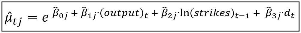
Mixing-in the Markov model
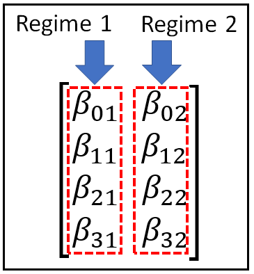
Now, let’s inject the impact of the 2-state Markov model. This causes all the regression coefficients β_cap=[β_cap_0, β_cap_1, β_cap_2, β_cap_3], and therefore the fitted mean μ_cap_t to become Markov state specific as shown below. Notice the additional subscript j that indicates the Markov state in effect at time t:
The corresponding Markov-specific Poisson probability of observing a particular count of strikes at time t given that the Markov state variable s_t is in state j at time t is as follows:
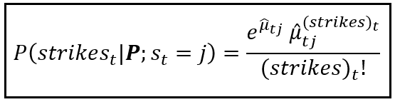
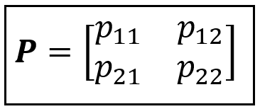
Where, the Markov state transition matrix P is:
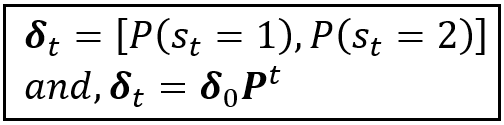
And the Markov state probability vector containing the state-wise probability distribution at time t is as follows:
With the above discussion in context, let’s restate the exogenous and endogenous variables of our Poisson Hidden Markov Model for the strikes data set:
Dependent variable (endogenous variable)
y = strikes
Regression variables (exogenous variables)
X = [output, ln (strikes_LAG_1), d_t] and P
Training and optimization
Training the Poisson PMM involves optimizing the Markov-state dependent matrix of regression coefficients (Note that in the Python code, we’ll work with the transpose of this matrix):
And also optimizing the state transition probabilities (the P matrix):
Optimization will be done via Maximum Likelihood Estimation where the optimizer will find the values of β and P which will maximize the likelihood of observing y. We will use the BFGS optimizer supplied by statsmodels to perform the optimization.
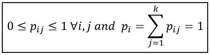
There is a little wrinkle that we need to smooth out. All throughout the optimization process, the Markov state transition probabilities p_ij need to obey the following constraints which say that all transition probabilities lie in the [0,1] interval and the probabilities across any row of P always sum to 1:
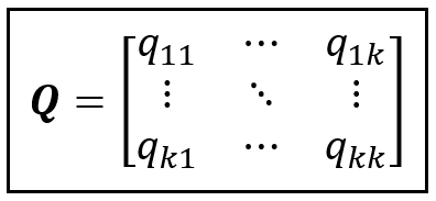
During optimization, we tackle these constraints by defining a matrix Q of size (k x k) that acts as a proxy for P as follows:
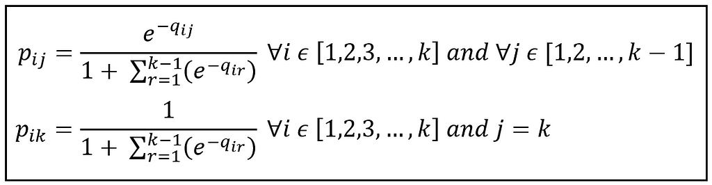
Instead of optimizing P, we will optimize Q by allowing q_ij to range freely from -∞ to +∞. In each optimization iteration, we obtain p_ij by standardizing the q values to the interval [0.0, 1.0], as follows:
With that, let’s circle back to our strikes data set.
Prepare the strikes data set for training
We saw that in the strikes time series, there is a strong correlation at lag-1, add the lag-1 copy of strikes as a regression variable.
strikes_data['strikes_lag1'] = strikes_data['strikes'].shift(1)
#Drop rows with empty cells created by the shift operation
strikes_data = strikes_data.dropna()
Create the indicator function for calculating the value of the indicator variable d1 as follows: if strikes == 0, d1 = 1, else d1 = 0.
def indicator_func(x):
    if x == 0:
        return 1
    else:
        return 0
Add the column for d1 into the Dataframe:
strikes_data['d1'] = strikes_data['strikes_lag1'].apply(indicator_func)
Adjust the lagged strikes variable so that it is set to 1, when its value is 0.
strikes_data['strikes_adj_lag1'] = np.maximum(1, strikes_data['strikes_lag1'])
Add the natural log of strikes_lag1 as a regression variable.
strikes_data['ln_strikes_adj_lag1'] = np.log(strikes_data['strikes_adj_lag1'])
Form the regression expression in Patsy syntax. There is no need to explicitly specify the regression intercept β_0. Patsy will automatically include a placeholder for it in X.
expr = 'strikes ~ output + ln_strikes_adj_lag1 + d1'
Use Patsy to carve out the y and X matrices.
y_train, X_train = dmatrices(expr, strikes_data, return_type='dataframe')
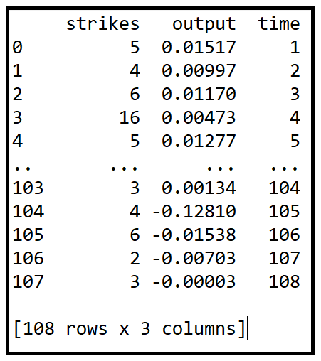
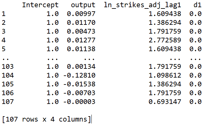
Let’s look at how our X and y matrices have turned out:
print(y_train)
print(X_train)
Before we get any further, we need to build the PoissonHMM class. For that we will use the statsmodels provided class GenericLikelihoodModel.
Create a Custom Poisson Hidden Markov Model class
The PoissonHMM class that we will create, will extend the GenericLikelihoodModel class so that we can train the model using a custom log-likelihood function. Let’s start by defining the constructor of the PoissonHMM class.
class PoissonHMM(GenericLikelihoodModel):
    def __init__(self, endog, exog, k_regimes=2, loglike=None,
                 score=None, hessian=None,
                 missing='none', extra_params_names=None, **kwds):
        super(PoissonHMM, self).__init__(endog=endog, exog=exog,
            loglike=loglike, score=score, hessian=hessian,
            missing=missing, extra_params_names=extra_params_names,
            kwds=kwds)
Now, let’s fill in the constructor i.e. the __init__ method of PoissonHMM with the following lines of code:
First, we’ll cast the dependent variable into a numpy array which statsmodels likes to work with. We’ll also copy over the number of regimes.
self.y = np.array(self.endog)
self.k_regimes = k_regimes
Next, set the k x m size matrix of regime specific regression coefficients β. m=self.exog.shape[1] being the number of regression coefficients including the intercept:
self.beta_matrix = np.ones([self.k_regimes, self.exog.shape[1]])
Set the k x k matrix of proxy transition probabilities matrix Q. Initialize it to 1.0/k.
self.q_matrix = np.ones([self.k_regimes,self.k_regimes])*(1.0/self.k_regimes)
print('self.q_matrix='+str(self.q_matrix))
Set the regime wise matrix of Poisson means. These would be updated during the optimization loop.
self.mu_matrix = []
Set the k x k matrix of the real Markov transition probabilities which will be calculated from the q-matrix using the standardization technique described earlier. Initialized to 1.0/k.
self.gamma_matrix = np.ones([self.k_regimes, self.k_regimes])*(1.0/self.k_regimes)
print('self.gamma_matrix='+str(self.gamma_matrix))
Set the Markov state probabilities (the π vector). But to avoid confusion with the regression model’s mean value which is also referred to as π, we will follow the convention used in Cameron and Trivedi and use the notation δ.
self.delta_matrix = np.ones([self.exog.shape[0],self.k_regimes])*(1.0/self.k_regimes)
print('self.delta_matrix='+str(self.delta_matrix))
Initialize the vector of initial values for the parameters β and Q that the optimizer will optimize.
self.start_params = np.repeat(np.ones(self.exog.shape[1]), repeats=self.k_regimes)
self.start_params = np.append(self.start_params, self.q_matrix.flatten())
print('self.start_params='+str(self.start_params))
Initialize a very tiny number that is machine specific. It is used by our custom Loglikelihood function which we will soon write.
self.EPS = np.MachAr().eps
Finally, initialize the optimizer’s iteration counter.
self.iter_num=0
The completed constructor of the PoissonHMM class looks like this:
Next, we will override the nloglikeobs(self, params) method of GenericLikelihoodModel. This method is called by the optimizer once in each iteration to get the current value of the loglikelihood function corresponding to the current values of all the params that are passed into it.
def nloglikeobs(self, params):
Let’s fill in this method with the following functions which we will define soon:
Reconstitute the Q and β matrices from the current values of all the params.
self.reconstitute_parameter_matrices(params)
Build the regime wise matrix of Poisson means.
self.compute_regime_specific_poisson_means()
Build the matrix of Markov transition probabilities by standardizing all the Q values to the 0 to 1 range.
self.compute_markov_transition_probabilities()
Build the (len(y) x k) matrix delta of Markov state probabilities distribution.
self.compute_markov_state_probabilities()
Compute the log-likelihood value for each observation. This function returns an array of size len(y) of loglikelihood values.
ll = self.compute_loglikelihood()
Increment the iteration count.
self.iter_num=self.iter_num+1
Print out the iteration summary.
print('ITER='+str(self.iter_num) + ' ll='+str(((-ll).sum(0)))
Finally, return the negated loglikelihood array.
return -ll
Here’s the entire nloglikeobs(self, params) method:
And following are the implementations of the helper methods called from the nloglikeobs(self, params) method:
Reconstitute the Q and β matrices from the current values of all the params:
Build the regime wise matrix of Poisson means:
Build the matrix of Markov transition probabilities P by standardizing all the Q values to the 0 to 1 range:
Build the (len(y) x k) size δ matrix of Markov state probabilities distribution.
Finally, compute all the log-likelihood values for the Poisson Markov model:
Let’s also override a method from the super class that tries its best to compute an invertible Hessian so that the standard errors and confidence intervals of all the trained parameters can be computed successfully.
def hessian(self, params):
    for approx_hess_func in [approx_hess3, approx_hess2,
                            approx_hess1]:
        H = approx_hess_func(x=params, f=self.loglike,
            epsilon=self.EPS)
        if np.linalg.cond(H) < 1 / self.EPS:
            print('Found invertible hessian using' +
                str(approx_hess_func))
            return H
    print('DID NOT find invertible hessian')
    H[H == 0.0] = self.EPS
    return H
Bringing it all together, here is the complete class definition of the PoissonHMM class:
Now that we have our custom PoissonHMM class in place, let’s get on with the task of training it on our (y_train, X_train) dataset of manufacturing strikes that we had carved out using Patsy.
Let’s recall how the constructor of PoissonHMM looks like:
def __init__(self, endog, exog, k_regimes=2, loglike=None,
            score=None, hessian=None, missing='none',
            extra_params_names=None, **kwds):
We’ll experiment with a 2-state HMM with the consequent assumption that the data cycles through 2 distinct but hidden regimes, each one of which influences the mean of the Poisson process. So we set k_regimes to 2:
k_regimes = 2
Notice that PoissonHMM takes an extra_param_names parameter. This is a list of parameters that we want the optimizer to optimize in addition to the column names of the X_train matrix. Let’s initialize and build this list of extra param names.
extra_params_names = []
There will len(X_train.columns) number of regression coefficients per regime to be sent into the model for optimization. So, in total, len(X_train.columns) * k_regimes β coefficients in all to be optimized. Out of which, the coefficients corresponding to one regime (say regime 1) are already baked into X_train in the form of the regression parameters. statsmodels will glean out their names from the X_train matrix. And it will automatically supply the names of this set of params to the model. So, we need to tell statsmodels the names of the remaining set of params via the extra_param_names parameter (hence the name extra_param_names), corresponding to the remaining regimes. Therefore, we insert the balance set of params for the 2nd regime into extra_param_names as follows:
for regime_num in range(1, k_regimes):
    for param_name in X_train.columns:
        extra_params_names.append(param_name+'_R'+str(regime_num))
The model will also optimize the k x k matrix of proxy transition probabilities: the Q matrix. So send those too into the extra_params list:
for i in range(k_regimes):
    for j in range(k_regimes):
        extra_params_names.append('q'+str(i)+str(j))
Note: In the Python code, we have chosen to work with 0 based indices for the Markov states. i.e. what we were referring to as state 1 is state 0 in the code.
Our list of extra_param_names is now ready.
Create an instance of the PoissonHMM model class.
poisson_hmm = PoissonHMM(endog=y_train, exog=X_train,
                        k_regimes=k_regimes,
                        extra_params_names=extra_params_names)
Train the model. Notice that we are asking statsmodels to use the BFGS optimizer.
poisson_hmm_results = poisson_hmm.fit(method=’bfgs’, maxiter=1000)
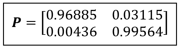
Print out the fitted Markov transition probabilities:
print(poisson_hmm.gamma_matrix)
We see the following output:
[[0.96884629 0.03115371]
 [0.0043594  0.9956406 ]]
Thus, our Markov state transition matrix P is as follows:
Which corresponds to the following state transition diagram:
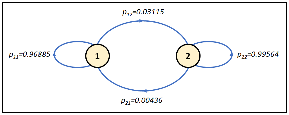
The state transition diagram shows that once the system gets into state 1 or 2, it really likes to be in that state and shows very little inclination to switch to the other state.
Finally, print out the model training summary:
print(poisson_hmm_results.summary())
We see the following output. I have called out the model’s parameters corresponding to the two Markov states 1 and 2, and the Q-matrix values (which happen to 0 indexed as noted earlier).
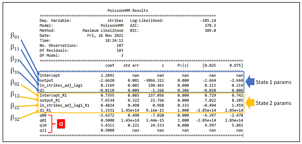
Here are a few things we observe in the output:
- The model fits to a different intercept in each one of the two Markov regimes. The intercept (β_0) is 2.2891 and 0.7355 in regimes 1 and 2 respectively.
- The effect of output (β_1) is -2.6620 in regime 1 indicating an inverse relationship between the growth of manufacturing output and number of strikes, and it is 7.6534 in regime 2 indicating as manufacturing output increases, so dothe incidence of strikes.
Goodness-of-fit
As we can see from the model training summary, the fit isn’t exactly fantastic as evidenced by the model’s inability to find valid standard errors for β_01 and q_11. And the params β_31, β_22, β_32 and q_01 are found to be not statistically significant as evidenced by their p-values.
Nevertheless, it is a good start.
To achieve a better fit, we may want to experiment with a 3 or 4 state Markov process and also experiment with another one of the large variety of optimizers supplied by statsmodels, such as ‘nm’ (Newton-Raphson), ‘powell’ and ‘basinhopping’.
Incidentally, since we are using the out-of-the-box method from statsmodels for printing the training summary, the df_model value of 3 printed in the training summary is misleading and should be ignored.
Lastly, it would be instructive to compare the goodness-of-fit of this model with that of the Poisson Auto-regressive model described here, and the Poisson INAR(1) model described here. All three models were fitted on the same manufacturing strikes data set:
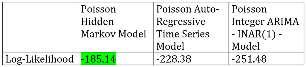
We can see that even after accounting for the much larger number of fitted parameters used by the Poisson HMM, the Poisson HMM model produces a much higher likelihood of observing the strikes data set values, than the other two kinds of time series models.
Where to go from here?
Here are some ways to build upon our work on the Poisson HMM:
- We could try to improve the fit of the PoissonHMM model class using a different optimizer and/or by introducing one more Markov state.
- We may want to calculate the pseudo-R-squared of the PoissonHMM class. The pseudo-R-squared provides an excellent way of comparing the goodness-of-fit of nonlinear models such as Poisson-HMM that are fitted on heteroskedastic datasets.
- Recollect that the Poisson model we have used assumes that the variance of strikes with any Markov regime is the same as mean value of strikes in that regime — a property kown as equidispersion. We can indirectly test this assumption by replacing the Poisson model with a Generalized Poisson or a Negative Binomial regression model. These models do not make the equidispersion assumption about the data. If a GP-HMM or an NB-HMM generates a better goodness-of-fit than the straight up Poisson-HMM, it makes a case for using those models.
Happy modeling!
Here is the complete source code:
Citations and Copyrights
Books
Cameron A. Colin, Trivedi Pravin K., Regression Analysis of Count Data, Econometric Society Monograph №30, Cambridge University Press, 1998. ISBN: 0521635675
Papers
Kennan J., The duration of contract strikes in U.S. manufacturing, Journal of Econometrics, Volume 28, Issue 1, 1985, Pages 5–28, ISSN 0304–4076, https://doi.org/10.1016/0304-4076(85)90064-8. PDF download link
Cameron C. A., Trivedi P. K., Regression-based tests for overdispersion in the Poisson model, Journal of Econometrics, Volume 46, Issue 3, 1990, Pages 347–364, ISSN 0304–4076, https://doi.org/10.1016/0304-4076(90)90014-K.
Data set
The Manufacturing strikes data set used in article is one of several data sets available for public use and experimentation in statistical software, most notably, over here as an R package. The data set has been made accessible for use in Python by Vincent Arel-Bundock via vincentarelbundock.github.io/rdatasets under a GPL v3 license.
Images
All images in this article are copyright Sachin Date under CC-BY-NC-SA, unless a different source and copyright are mentioned underneath the image.
Related Articles
- A Beginner’s Guide to Discrete Time Markov Chains
- A Math Lover’s Guide to Hidden Markov Models
- A Worm’s Eye-View of the Markov Switching Dynamic Regression Model
Thanks for reading! If you liked this article, please follow me to receive tips, how-tos and programming advice on regression and time series analysis.
How to Build a Poisson Hidden Markov Model Using Python and Statsmodels was originally published in Towards Data Science on Medium, where people are continuing the conversation by highlighting and responding to this story.
from Towards Data Science - Medium https://ift.tt/31yaKze
via RiYo Analytics


ليست هناك تعليقات