https://ift.tt/3FM7CyG Fundamentals Unlocking a key element of eigendecomposition Photo by Ricardo Gomez Angel on Unsplash There are...
Fundamentals
Unlocking a key element of eigendecomposition

There are concepts in linear algebra that are easy to understand the first time they come around. Probably, because their applications and use-cases are relatively obvious and the concepts are somewhat tangible.
The concept of the matrix determinant, however, did the complete opposite for me — I was more confused than enlightened. My confusion mainly stemmed from the fact, that I had a severe lack of intuition — I couldn’t visualize or imagine the meaning and the purpose of the determinant.
In the following sections, we are going to build some of that intuition, learn a few of the procedures to calculate the determinant, and get a first idea of its applications.
Quick facts and intuition
The determinant describes a function that maps matrices to a scalar. It is defined by the product of all eigenvalues, allowing for a slightly less abstract, more geometric interpretation.
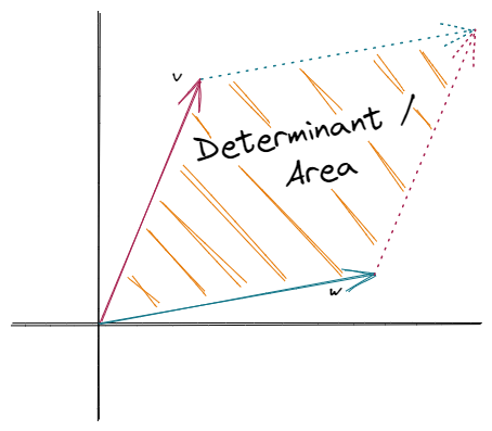
Depending on the matrix’s dimensions, the determinant can also be interpreted as the area or the volume respectively. Loosely speaking, it tells us how much the multiplication by that given matrix stretches or shrinks space.

Suppose we have a matrix with a determinant of zero. Multiplication by that matrix, will contract space and squish everything onto a single line. Therefore, the area will equal zero as well.
Now, that we gained some basic intuition, we can list some facts about the determinant to further our understanding:
- The determinant is only defined for square matrices (M x M).
- A matrix has exactly one determinant, since it is a scalar, containing information about the matrix.
- The determinant equals zero for singular matrices. Or put differently — matrices with linear dependencies, rank r < M, have a determinant of zero.
- The determinant will often be denoted as one of the following:

Note: One thing to keep in mind — the determinant is great in theory but hard to compute in practice, due to numerical instabilities when calculated for ‘large’ matrices.
How to compute the matrix determinant?
In the previous section, we learned some basic facts about the determinant and how to interpret it. But how do we calculate it?
The procedure to calculate the determinant is quite tedious. Fortunately, there exist some shortcuts, which are only applicable to small matrices (2x2, 3x3). We will talk about the shortcuts first, before talking about the general procedure.
Note: Luckily, we don’t have to calculate the determinant manually, since the built-in NumPy function numpy.linalg.det(a) will do the job for us.
2x2 shortcut
The determinant for a 2 by 2 matrix is relatively easy to compute. We just have to multiply every element along the main-diagonal and subtract the product of the off-diagonal elements.

Let’s work through some numerical examples:


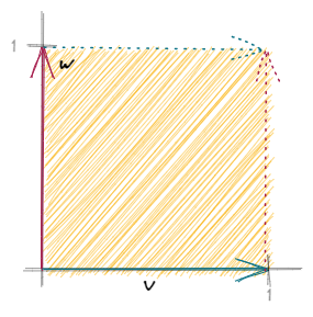
In the first example, we used the shortcut to calculate the determinant of a 2 by 2 identity matrix, which equals one. We can also visualize this solution as the area of a plane, where one side is defined by the unit vector v=[1, 0] and the other by the unit vector w=[0, 1].

A singular matrix has a determinant of zero — and this is exactly, what we can see in our second example. Since both columns are linear dependent on each other, we have a rank-deficient matrix, resulting in a determinant of zero. Thinking about the solution more geometrically, we have to imagine two vectors forming just a single line with an area of zero.

3x3 shortcut
The computation of the determinant for a 3 by 3 matrix is already more involved, but relatively similar to the 2 by 2 shortcut.

We sum all the products of the diagonal elements from top-left to bottom-right and subtract the sum of all the products of the off-diagonal elements from top-right to bottom-left. We can visualize this procedure in two different ways.
- One way is to augment the matrix by concatenation:

2. The other way is to imagine a ‘wrap around’ along the diagonals:

General procedure
Now, it gets complicated really quickly. Thus, the following example will only be based on a 4 by 4 matrix.
In general, the procedure is to iterate over each element of the first row, create a submatrix (3x3) by excluding the column of the current first-row element, calculate the determinant of the submatrix and multiply by the current first-row element. This will yield four numbers, which we will add and subtract in an alternating pattern [+,-,+,-].
We should visualize the procedure to untangle the complicated description:

We can see the procedure is a lot more involved. For a relatively small 4 by 4 matrix, we have to compute 4 determinants of 4 submatrices, of which we also need to compute the determinants of the submatrices, etc. So the algorithm can be applied recursively and thus gets computationally expensive.
This general procedure, however, can scale up to any sized matrix — and fortunately, we don’t have to calculate it by hand.
Applications of the determinant
We know now what the determinant is, how to interpret it, and how to calculate it, but one question still remains unanswered — What is it used for?
Some of its applications are, for example, providing a way to find the inverse of a given matrix or to find the eigenvalues. The latter is especially important, since eigenvalues and thus eigendecomposition play a central role in the principal component analysis.
Assume we have a 2 by 2 matrix and we already know the determinant. Putting the matrix elements on one side and the determinant on the other side of an equation, allows us to solve for a particular element of the matrix.
Let’s think about a numerical example to make things a bit more obvious.


Now, if we build on this idea and subtract multiple unknowns from real numbers across the main-diagonal and generalize the equation, we obtain the characteristic polynomial of the matrix.

The characteristic polynomial is useful, since it allows us not only to express a matrix in terms of a polynomial expression but also to compute the eigenvalues of a matrix. If the characteristic polynomial is set to zero, the λ’s — which are the roots of the polynomial — describe the eigenvalues of the matrix.
Conclusion
In this article, we learned about the concept of the matrix determinant. How to interpret and calculate it, as well as some of its applications.
Two of the most important applications are the calculation of the matrix inverse and perhaps even more interesting, the discovery of the eigenvalues.
As we briefly touched upon earlier, the matrix determinant is a great concept in theory, but hard to compute in practice, especially for ‘large’ matrices due to numerical instabilities. To avoid such issues, when for example calculating the eigenvalues, a whole family of iterative algorithms (e.g. the power method) exist.
Despite the practical issues, the determinant is still a great and fundamental concept to know and understand.
Thank you for reading! Make sure to stay connected & follow me here on Medium, Kaggle, or just say ‘Hi’ on LinkedIn
References / Further Material:
- Deep Learning (Ian J. Goodfellow, Yoshua Bengio and Aaron Courville), Chapter 2, MIT Press, 2016.
- Mike X Cohen, PhD. Linear Algebra: Theory, Intuition, Code.
- 3Blue1Brown — The Determinant
Discovering The Matrix Determinant was originally published in Towards Data Science on Medium, where people are continuing the conversation by highlighting and responding to this story.
from Towards Data Science - Medium https://ift.tt/3HtDVmr
via RiYo Analytics

ليست هناك تعليقات