https://ift.tt/3FuAE5v Why domain scientists know more ML than they think Maxim Ziatdinov¹ ² & Sergei V. Kalinin¹ ¹ Center for Nanoph...
Why domain scientists know more ML than they think
Maxim Ziatdinov¹ ² & Sergei V. Kalinin¹
¹ Center for Nanophase Materials Sciences and ² Computational Sciences and Engineering Division, Oak Ridge National Laboratory, Oak Ridge, TN 37831, United States
About 20 years ago, Donald Rumsfeld, the erstwhile minister of defense, famously said referring to the intelligence situation, “…there are known knowns; there are things we know we know. We also know there are known unknowns; that is to say we know there are some things we do not know. But there are also unknown unknowns — the ones we don’t know we don’t know.”. Despite coming from a different context, this statement profoundly describes the work of scientists. We establish our worldview and build fundamental exploration based on what we know, can read in the textbooks, or have learned throughout our professional career from experience, discussions with colleagues, or spending countless hours in the labs. These are the known knowns. We also often know what we do not know — and typically, these known unknowns are the immediate target of our research. That said, for each scientific experiment, the unknown unknowns are critical — the factors outside of our sphere of attention that can drastically affect our measurements, analyses, and conclusions.
Obviously, the very succinct statement by Rumsfeld is not the first time the division of the world into types of knowns and unknowns was noticed. To the authors’ knowledge, the first documented statement to this effect can be traced to Naser od-Din Tusi (1201–1274), who said
Har kas ke bedanad va bedanad ke bedanad
Asb-e kherad az gombad-e gardun bejahanad
Har kas ke nadanad va bedanad ke nadanad
Langan kharak-e khish be manzel beresanad
Har kas ke nadanad va nadanad ke nadanad
Dar jahl-e morakkab’abad od-dar bemanad
or, in translation from Farsi:
Anyone who knows, and knows that he knows
Makes the steed of intelligence leap over the vault of heaven
Anyone who does not know, but knows that he does not know
Can bring his lame little donkey to the destination nonetheless
Anyone who does not know, and does not know that he does not know
Is stuck forever in the double ignorance
It is highly possible that the historical references can go even earlier, but we were unable to find them. That said, despite the significant progress of the instruments of scientific inquiry from the Abbasid and Umayyad eras, the role of the known and unknown factors in scientific discovery remains.
For example, in his scientific career the second author worked extensively with Electrochemical Strain Microscopy (ESM), the technique that allows probing electrochemical reactions on the nanometer level via measuring minute (smaller than the radius of the hydrogen atom) expansion and contraction of material induced by ionic motion [1, 2]. The measured signal in the ESM is a local hysteresis loop, representing the electrochemical response of a material to bias. For a classical material such as ceria CeO₂, these hysteresis loops will be very reproducible between distinct locations on the sample surface. This suggests that they are descriptive of the reactions at the scanning probe microscopy tip-surface junction and are not affected by the possible variations of materials composition (we did not expect much) or surface roughness (which is always a problem in SPM). However, the shape of the hysteresis loops changed completely when the measurements were performed in a controlled gas atmosphere and, yet again, vacuum. And this, in turn, signified that the atmospheric environment is a significant factor in the measured responses. If we had not done the measurements in several atmospheres (that required non-standard modifications to the microscope) and tried to describe the mechanisms without considering the role of atmospheric water, this would have been a typical example of an unknown unknown. As it were, it became a known unknown — which stimulated another decade of theoretical and experimental studies and led to the discovery of unusual coupling between ferroelectricity and surface electrochemistry [3], among other developments.
That said, are the three categories of knowns/unknows all there is to it? We pose that when actively incorporating machine learning methods into the domain science, we often discover unknown knowns — meaning the full spectrum of prior knowledge ranging from generalizations (physical laws) and domain-specific data, all the way to the difficult-to-quantify intuition. Hence, the question now becomes, how can we incorporate the prior knowledge, the unknown knowns, into the scientific discovery process and do so in a principled and quantifiable manner.
The general framework for this is laid by the Bayes formula. There are multiple excellent books describing the Bayesian approach, as well as Medium posts. For the second author, the preferred point of entry into all things Bayesian were the books by Martin [4] and Lambert [5], with the systematic comparison between Bayesian and frequentist methods given by Kruschke [6] The first author believes that the best (for the domain scientist) book on the Bayesian analysis is Richard McElreath’s “Statistical Rethinking”.
Below, we give the classical Bayes formula from the domain scientist perspective. Here, the purpose of the scientific experiment is to derive new knowledge, aka probability of theory, from the newly acquired experimental data.
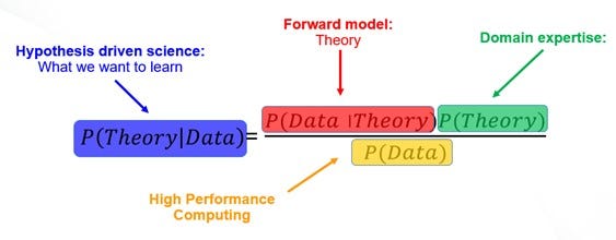
Here, the probability of data given the theory, or likelihood in Bayesian language, is directly accessed using the forward modeling. The probability of data, or evidence, is directly assessed using computational methods, whether it is Markov Chain Monte Carlo or Variational Inference. But it is the third part — the probability of theory, or a prior — that typically raises most issues. Indeed, the critique often leveled at Bayesian models is that they require priors, and these are difficult to be established consistently. And in fact, they are — if one stays fully in the statistics field. For a domain expert, prior knowledge is absolutely essential and actually defines domain expertise. However, it is the unknown known, and very often this knowledge is not easy to quantify or establish in the form of prior distributions in the traceable algorithmic form. Perhaps even more importantly, it is not immediately clear how to incorporate the prior knowledge in the active learning workflows for experimental discovery. Let’s consider them one by one.
Once the experimental data is available, the Bayesian Inference methods allow straightforward analytics to be performed. For example, recently, we have explored the structure of ferroelectric domain walls using high-resolution electron microscopy [7]. Here, the domain wall structure is determined by the specific functional form of the free energy that gives rise to analytical solutions describing the domain wall profile. The simple functional fits, as done earlier [8, 9], give numerical estimates of the parameters, but do not allow to go beyond these. Comparatively, Bayesian methods allow incorporating the prior knowledge of materials’ physics in the form of prior distributions of relative constants, which in turn can be obtained from the preponderance of published data, macroscopic measurements, etc. For example, one of the values of large materials informatics projects such as Materials Project is that it integrates the data from multiple separated sources into easy-to-access form.
Similarly, the Bayesian framework allows answering non-trivial questions such as whether prior knowledge of materials physics affects what we learn from the experiment (quite surprisingly — the more we know, the more we learn), whether the specific models of materials behaviors can be differentiated based on the observed data (not in this case), and what microscope resolution or information limit is necessary to distinguish different models. Similarly, Bayesian methods allow defining many “absolute” quantities in a probabilistic fashion — for example, descriptors such as symmetry or structural units [10].
However, the next question becomes whether we can use the Bayesian approach for active learning and property optimization? In principle, it is possible to use the classical Bayesian approach as detailed above. Here, we define the prior hypothesis as a structured probabilistic model. Given the experimental data, we refine the parameters of our model and then explore the posterior predictive probabilities over the parameter space. Much like classical Bayesian Optimization/active learning (BO/AL) described in our previous post, the expected value and/or associated uncertainty can be used to guide the measurements (i.e., select the next measurement point).
However, practically, the BO/AL based on the structured probabilistic model of the expected system’s behavior does not work well when the model is only partially correct. At the same time, this is exactly what we usually have to deal with in experiments where even the most sophisticated theory describes reality only to a certain approximation, and several competing models are possible, not to mention all the measurements-related non-idealities. Of course, the alternative is to substitute a rigid structured probabilistic model with a highly flexible Gaussian process (GP). The latter, however, does not usually allow for the incorporation of prior domain knowledge and can be biased toward a trivial interpolative solution.
Hence, we introduce a structured Gaussian Process (sGP), where a classical GP is augmented by a structured probabilistic model of the expected system’s behavior [11]. This approach allows us to balance the flexibility of the non-parametric GP approach with a rigid structure of prior (physical) knowledge encoded into the parametric model. The Bayesian treatment of the latter provides additional control over the BO/AL via the selection of priors for the model parameters, i.e., incorporation of the past knowledge.
More formally, given the input parameters x and target property y, the classical GP is defined as y ~ MultivariateNormal(m(x), K(x, x`)), where m is a mean function usually set to 0 and K is a kernel function with weakly-informative priors (usually chosen as LogNormal) over its parameters. The latter can be inferred using the Hamiltonian Monte Carlo (HMC) sampling technique. Then, the prediction on the new/unmeasured set of inputs is given by
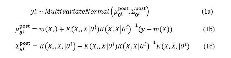
where θⁱ is a single HMC posterior sample with kernel hyperparameters. Note that the commonly assumed observation noise is absorbed into the computation of the kernel function. (We denoted the new inputs and associated prediction by a * subscript — unfortunately, at the moment of writing, the Medium does not have the in-line support for this and other subscripts).
In our sGP approach, we substitute a constant mean function m in the equations above with a structured probabilistic model whose parameters are inferred together with the kernel parameters via the HMC. Then, the Eq (1b) becomes:
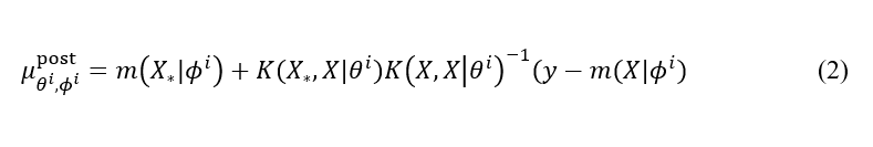
where ϕⁱ is a single HMC posterior sample with the learned model parameters. This probabilistic model reflects our prior knowledge about the system, but it does not have to be precise, that is, the model can have a different functional form, as long as it captures general or partial trends in the data.
Bayesian Optimization with structured GP
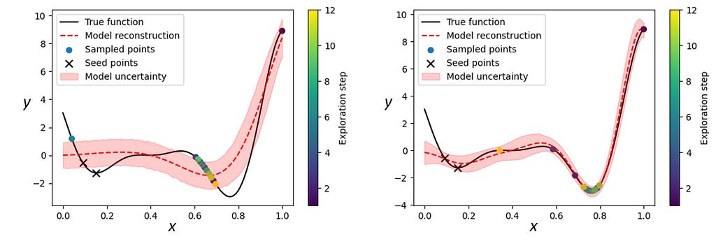
We will illustrate the advantage of the sGP approach with specific examples. First, we are going to use a slightly modified Forrester function, f(x) = (5x-2)²sin(12x-4), which is commonly used to evaluate the optimization algorithms. It has two local minima in addition to the global minimum. Our goal is to converge on the global minimum using only a small number of steps (measurements). First, we use BO with vanilla GP. We start with a ‘good’ initialization of the seed points (the ‘warmup’ measurements performed before running the BO) and use the upper confidence bound (UCB) acquisition function with k = -0.5, for selecting the next measurement point at each step. As expected, the GP-BO quickly converged on the true minimum.
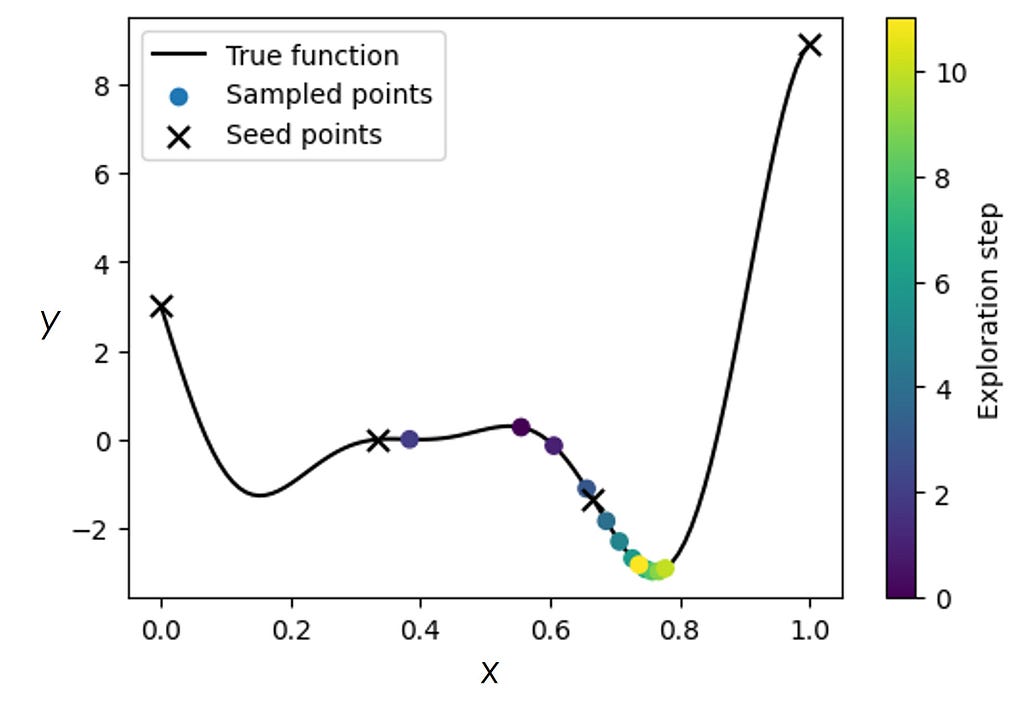
Now, let’s start with a ‘bad’ initialization where the initialized points fall into the region around one of the local minima. Due to this bad initialization, the GP-BO gets stuck in a local minimum and is unable to converge on the true minimum. We note that in the real experiments, one does not usually have the luxury of restarting measurements using different initializations, and therefore must be equipped to deal with bad initializations.
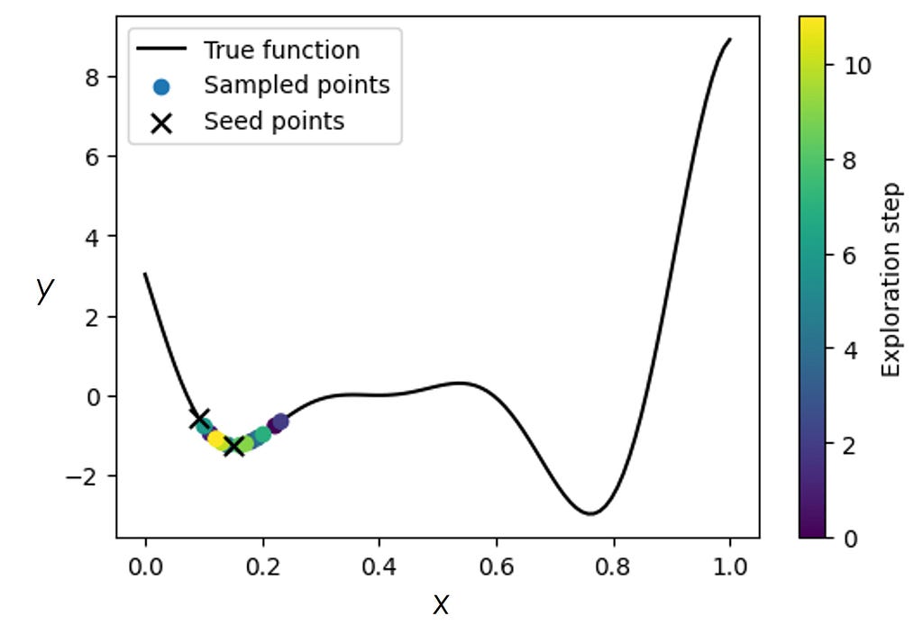
One way to look at the example above is that we got stuck in a local minimum because our algorithm did not “know” about the potential existence of a different minimum. But if we do know that there may be more minima (one of which could be the true/global one), then this prior knowledge can be incorporated into the sGP model.
Specifically, let’s define a structured probabilistic model as
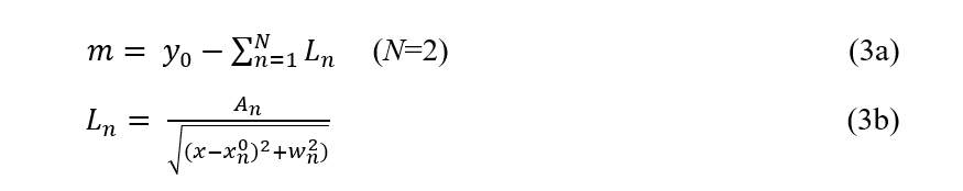
where y₀ ~ Uniform(-10, 10), Aₙ ~ LogNormal(0, 1), wₙ ~ HalfNormal(0.1), and xₙ⁰ ~ Uniform(0, 1) are the priors over the model parameters. This model simply tells us that there are two minima in our data but does not assume to have any knowledge about their relative depth and width, nor does it contain information about how far apart they are. We then substitute the constant prior mean function m in GP with the probabilistic model defined in Eq (3) and run the BO for the ‘bad’ initialization the same way as before.
We can see that the optimization algorithm equipped with some knowledge of the expected system’s behavior was able to pull itself away from a local minimum and converge onto the global one. We have performed a systematic comparison between GP-BO and sGP-BO for several dozens of different random initializations of the seed points and in the presence of noise and found a superior performance of the sGP-BO in nearly all cases [11].
To understand the superior performance of the sGP-BO, we can compare the acquisition functions for GP-BO and sGP-BO at different steps of the optimization.
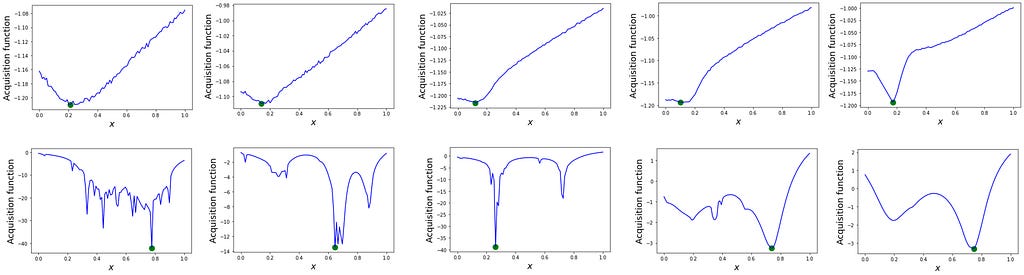
Clearly, the vanilla GP-BO gets quickly locked in a local minimum with its acquisition function remaining largely unchanged (top row in Figure 5) as the algorithm ‘assumes’ it already found the true/global minimum. On the other hand, the acquisition function in the sGP-BO (bottom row in figure 5) displays a structure with multiple minima early on, which helps the algorithm to climb out of the local minimum and to converge on the true minimum at the later steps of the process even despite a very bad initialization. The evolution of the acquisition function in the bottom row of Figure 5 is truly remarkable in the sense that the algorithm is looking for a second minimum as if driven by intuition. And in some sense, it is— the prior knowledge we incorporated in the form of GP’s mean function in Eq (3) postulates that there is a second minimum somewhere — and the acquisition function highlights where this second minimum is most likely to be.
But what if this “prior knowledge” is only partially correct? As noted earlier, the advantage of sGP-BO compared to standalone probabilistic models is that the flexibility of the GP kernel allows us to use imprecise and sometimes even ‘incorrect’ functional forms of the models. We illustrate this using a structured probabilistic model of the form m = Aeᵃˣsin(bx), with (log)normal priors on its parameters, for BO as a standalone model and as a part of sGP. We note that while this is clearly not the right model for describing the Forrester function, it does nevertheless capture some trends in data such as the presence of a global minimum and multiple local minima.
The BO with a standalone probabilistic model (Figure 6, left) was not able to converge on the global minimum. The inference per se is too rigid and fails if the reality does not fit into the chosen model framework. It also could not produce a satisfactory reconstruction of the objective function even around the measured points and its uncertainty estimates do not appear to be particularly meaningful. On the other hand, the sGP-BO with the same probabilistic model as a part of the GP, easily identified the true minimum (Fig. 6, right). It also performed a good reconstruction of the underlying function around the measured regions and provided meaningful uncertainty estimates outside those regions, which could be used to select the next measurement points for a full recovery of the objective function (if necessary).
Structured GP for actively learning discontinuous functions
As our second example, we show how sGP can be used to reconstruct a discontinuous function from sparse and noisy observations. We note that the presence of discontinuities is common in the physics of phase transitions where one typically wants to reconstruct the behavior of the property of interest close to the transition point as well as in two phases before and after the transition. At the same time, the standard GP is not equipped to work with such discontinuities.
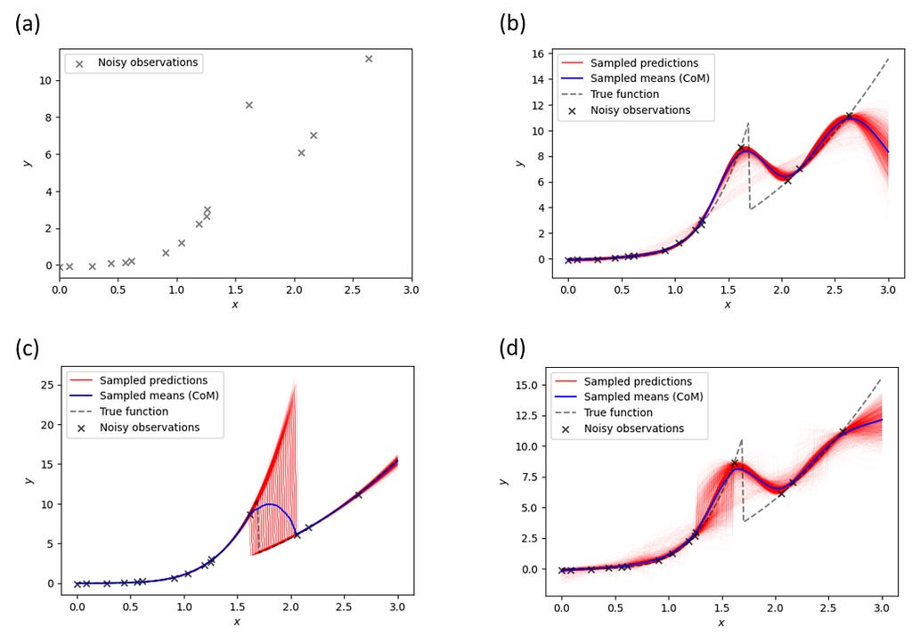
Figure 7a shows observations generated by the piecewise function of the form

Our goal is to reconstruct the underlying function from these noisy data points. First, we try vanilla GP (Figure 7b). It doesn’t perform well, which should not be very surprising since the standard GP is not equipped to deal with discontinuities. Intuitively, it can be understood by the contradictory requirements the discontinuity brings to the kernel function — the kernel with a large length scale cannot describe discontinuity, whereas small length scales necessitate multiple measurements to discover function behavior everywhere. Note that simple GP also extrapolates poorly outside the measurement interval (albeit in this case multiple strategies to address this issue are available).
Next, we try the sGP augmented by two different probabilistic models. The first sGP is augmented by a piecewise probabilistic function that has a general power-law form of axᵇ for x < xₜ and cxᵈ for x ≥ xₜ, with a uniform prior on xₜ and log-normal priors on the other parameters. It shows a good overall reconstruction (Figure 7c) except for the transition region where we do not have enough observations. However, this region is also characterized by very large uncertainty (variation in the sampled predictions), suggesting that one may want to perform extra measurements in that area. It is also remarkable to examine the behavior of sampled predictions in this case — essentially, they differ in estimation on where the switch point is located. Again, this comports to the scientist's decision-making logic— if we expect the phase transition and are confident in the functional behavior of measured response before and after the transition, the only remaining uncertainty is the transition point!
The second sGP is augmented by a piecewise probabilistic function equal to ax for x < xₜ and bx for x ≥ xₜ, with a uniform prior on xₜ and log-normal priors on the a and b. Note that this model is only partially correct: it has a transition point but assumes linear (instead of power-law) behavior before and after the transition. As a result, the reconstruction quality (Figure 7d) is lower, even though it is still somewhat better than for vanilla GP. Note that in this case the maximal uncertainty is associated with behavior before the transition (we do not expect the power-law behavior).
The uncertainties in the model predictions can be used to guide measurements to obtain a more accurate reconstruction of the underlying function. The procedure is the same as in the Bayesian optimization, except that we use the model’s uncertainty instead of the acquisition function to predict the next measurement point.
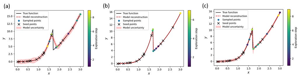
We can see that both sGP models quickly focused on the transition region before exploring other parts of the parameter ‘space’ (Figure 8b, c). As a result, we were able to improve dramatically the quality of the reconstruction. On the other hand, the uncertainty-guided exploration with vanilla GP still failed to reconstruct the transition region (Figure 8a). Hence, we see again that even sGP with a partially correct model of the expected system’s behavior can outperform the standard GP approach.
In summary, the augmentation of the Gaussian process with a (fully Bayesian) probabilistic model of the expected system’s behavior allows for more efficient optimization and active learning of a system’s properties. Note that even for incorrect or partially correct models the active learning algorithm will eventually arrive at the right answer — but at the cost of a larger number of experimental steps. Check our preprint for more details, including the application of this concept to physical models [11]. Please also check out our gpax software package for applying this and other GP tools to scientific data analysis. If you want to learn more about the Scanning Probe Microscopy, you are welcome to the channel M*N: Microscopy, Machine Learning, Materials.
Finally, in the scientific world, we acknowledge our research sponsor. This effort was performed and supported at Oak Ridge National Laboratory’s Center for Nanophase Materials Sciences (CNMS), a U.S. Department of Energy, Office of Science User Facility. You can take a virtual walk through it using this link and please let us know if you want to know more.
The executable Google Colab notebook is available here.
References:
1. Balke, N.; Jesse, S.; Morozovska, A. N.; Eliseev, E.; Chung, D. W.; Kim, Y.; Adamczyk, L.; Garcia, R. E.; Dudney, N.; Kalinin, S. V., Nanoscale mapping of ion diffusion in a lithium-ion battery cathode. Nat. Nanotechnol. 2010, 5 (10), 749–754.
2. Kumar, A.; Ciucci, F.; Morozovska, A. N.; Kalinin, S. V.; Jesse, S., Measuring oxygen reduction/evolution reactions on the nanoscale. Nat. Chem. 2011, 3 (9), 707–713.
3. Yang, S. M.; Morozovska, A. N.; Kumar, R.; Eliseev, E. A.; Cao, Y.; Mazet, L.; Balke, N.; Jesse, S.; Vasudevan, R. K.; Dubourdieu, C.; Kalinin, S. V., Mixed electrochemical-ferroelectric states in nanoscale ferroelectrics. Nature Physics 2017, 13 (8), 812–818.
4. Martin, O., Bayesian Analysis with Python: Introduction to statistical modeling and probabilistic programming using PyMC3 and ArviZ, 2nd Edition. Packt Publishing: 2018.
5. Lambert, B., A Student’s Guide to Bayesian Statistics. SAGE Publications Ltd; 1 edition: 2018.
6. Kruschke, J., Doing Bayesian Data Analysis: A Tutorial with R, JAGS, and Stan. Academic Press; 2 edition: 2014.
7. Nelson, C. T.; Vasudevan, R. K.; Zhang, X. H.; Ziatdinov, M.; Eliseev, E. A.; Takeuchi, I.; Morozovska, A. N.; Kalinin, S. V., Exploring physics of ferroelectric domain walls via Bayesian analysis of atomically resolved STEM data. Nat. Commun. 2020, 11 (1), 12.
8. Borisevich, A. Y.; Morozovska, A. N.; Kim, Y. M.; Leonard, D.; Oxley, M. P.; Biegalski, M. D.; Eliseev, E. A.; Kalinin, S. V., Exploring Mesoscopic Physics of Vacancy-Ordered Systems through Atomic Scale Observations of Topological Defects. Phys. Rev. Lett. 2012, 109 (6).
9. Li, Q.; Nelson, C. T.; Hsu, S. L.; Damodaran, A. R.; Li, L. L.; Yadav, A. K.; McCarter, M.; Martin, L. W.; Ramesh, R.; Kalinin, S. V., Quantification of flexoelectricity in PbTiO3/SrTiO3 superlattice polar vortices using machine learning and phase-field modeling. Nat. Commun. 2017, 8.
10. Kalinin, S. V.; Oxley, M. P.; Valleti, M.; Zhang, J.; Hermann, R. P.; Zheng, H.; Zhang, W.; Eres, G.; Vasudevan, R. K.; Ziatdinov, M., Deep Bayesian local crystallography. npj Computational Materials 2021, 7 (1), 181.
11. Ziatdinov, M. A.; Ghosh, A.; Kalinin, S. V., Physics makes the difference: Bayesian optimization and active learning via augmented Gaussian process. arXiv:2108.10280 2021.
Unknown Knowns, Bayesian Inference, and structured Gaussian Processes was originally published in Towards Data Science on Medium, where people are continuing the conversation by highlighting and responding to this story.
from Towards Data Science - Medium https://ift.tt/3Fo5v3A
via RiYo Analytics


No comments