https://ift.tt/3DPijzT A Practical Guide to ARIMA Models using PyCaret — Part 1 Laying the Statistical Foundations Photo by Agê Barros ...
A Practical Guide to ARIMA Models using PyCaret — Part 1
Laying the Statistical Foundations

📚 Introduction
PyCaret is an open-source, low-code machine learning library in Python that automates machine learning workflows. It is an end-to-end machine learning and model management tool that speeds up the experiment cycle exponentially and makes you more productive.
PyCaret recently released a Time Series Module which comes with a lot of handy features that make time series modeling a breeze. You can read more about it in this article.
📢 Announcing PyCaret’s New Time Series Module
In this multi-part series of articles, we will focus on how we can use a “low-code” library like PyCaret to get a deeper understanding of the working of the ARIMA model. In part 1, we will look at an overview of the ARIMA model and its parameters. Then, we will start with a simple ARIMA model and create a theoretical framework for this model’s predictions and the prediction intervals to develop intuition about its working. Finally, we will build this ARIMA model using PyCaret and compare the theoretical calculation to the models output. Correlation of the model’s output to our theoretical framework will hopefully bolster our understating of the model and lay the foundation for more detailed analysis in subsequent articles.
📖 Suggested Previous Reads
This article is recommended for those who have a basic understanding of time series (for example, concepts like seasonality, auto-correlation ACF, white noise, train-test-split) but are interested in knowing more about the ARIMA model. If you are not familiar with these concepts, I would recommend going through these short reads first. This will help ease into this article.
👉 Seasonality and Auto Correlation in Time Series
👉 Time Series Cross Validation
1️⃣ ARIMA Model Overview
ARIMA is a classical time series model that models the auto-regressive properties of temporal data. Auto-regressive means something that depends on past values of itself. A time series could depend on (1) its immediate past value or (2) may exhibit seasonal behavior and repeat itself after a certain number of time points have elapsed.
Intuitively, an example of (1) is stock data. This is temporal data where the price tomorrow is heavily influenced by the price today (or recent past) and not so much with what happened one month or one year back. Similarly, an example of (2) could be sales of winter clothes in a retail store. This usually peaks right before the winter months and dies down in summer months. Hence it exhibits a seasonal pattern. The sales in winter this year will be highly correlated to the sales in winter of last year.
Now that we have seen some basic examples, let’s see how this is represented in a model. The classical ARIMA model has several hyperparameters, but we will focus on the 2 main ones — order, and seasonal_order.
order:
iterable or array-like, shape=(3,), optional (default=(1, 0, 0))
The (p,d,q) order of the model for the number of AR parameters,     differences, and MA parameters to use.
seasonal_order:
array-like, shape=(4,), optional (default=(0, 0, 0, 0))
The (P,D,Q,s) order of the seasonal component of the model for the     AR parameters, differences, MA parameters, and periodicity.
Now, you may be wondering how these terms correlate to the examples we highlighted above and what the three and four terms in order and seasonal_order respectively mean. At a very high level, order relates to example (1) above where the next value is strongly correlated to the immediate previous value(s). seasonal_order relates to example (2) above where the next value is related to the data from one or more seasons back in time.
But that still does not answer the question what is (p, d, q) and (P, D, Q, s) . That is exactly what we will try to answer in these series of articles.
NOTE: This series of articles takes a “code first” approach to understanding the ARIMA model. I would highly recommend that readers also refer to [5] for a better understanding from a theoretical perspective.
2️⃣ Baseline ARIMA Model
To get a better understanding of the various hyperparameters of the ARIMA model, let’s start with a very simple ARIMA model — one that does not have any auto regressive properties. This is usually used to represent white noise (i.e. data that does not have any signal in it). You can find more information about it in [1] and [2]. This model is represented with the following hyperparameters:
##############################################
#### Baseline ARIMA Model Hyperparameters ####
##############################################
(p, d, q)    = (0, 0, 0)
(P, D, Q, s) = (0, 0, 0, 0)
Theoretically, since the time series data does not have any signal, the best representation of future predictions (out of sample) is the mean of the data used to train the model (see [2] for details). Similarly, the best estimate of in-sample predictions is also the mean of the data used to train the model.
We can get the prediction interval for these predictions by computing the residuals of the in-sample fit. The residuals represent the difference between the actual in-sample data (i.e. data used for training) and the in-sample estimate produced by this model (mean of training data in this case).
OK, so theory is one thing, but a picture is worth a thousand words. So let’s put this to practice. We will use PyCaret’s Time Series Module to get a deeper understanding of this model. Note that a notebook for the code can be found here and in the Resources section.
3️⃣ Understanding the ARIMA model using PyCaret
PyCaret’s time series module provides a data playground of over 2000 time series with known properties. We will use a “white noise” dataset from this playground to explain this example.
👉 Step 1: Setup PyCaret Time Series Experiment
#### Get data from data playground ----
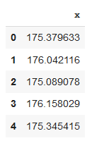
y = get_data("1", folder="time_series/white_noise")
Next, let’s setup a Time Series Experiment to explore and model this dataset. The “Time Series Experiment” is a one stop shop where a user can perform exploratory analysis (EDA), model building, model fit assessment as well as deployment — all while following best modeling practices under the hood.
In this setup, I set the forecast horizon fh to 30 (i.e. we intent to forecast the next 30 time points). I also set the seasonal_period to 1 for now. Note, if your data has a DatetimeIndex or PeriodIndex index (which is not the case here), then the seasonal period is auto inferred. If it is an anything else, we need to pass the seasonal period. I also passed a session ID which acts as a seed and makes the experiment reproducible.
#### Setup experiment ----
exp = TimeSeriesExperiment()
exp.setup(data=y, seasonal_period=1, fh=30, session_id=42)
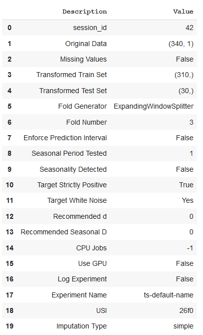
The setup provides some handy information to us right from the start.
(1) We see that our data has 340 data points. For this experiment, pycaret kept the last 30 (same as the forecast horizon) as a “test set” and the remaining 310 data points are used or training.
(2) We passed a seasonal period of 1, but after internally testing for seasonality, it was not detected. This is as expected since this is white noise data that does not have seasonality.
(3) A Ljung-Box test for White Noise (see previous reads) was done internally and it was determined that the data is consistent with white noise. Again, this is what we would expect since we picked the data from the white noise playground.
👉 Step 2: Perform EDA
Next, we can do quick EDA on this data:
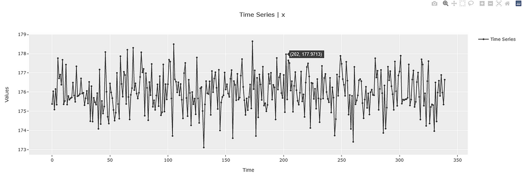
# `plot_model` without any estimator works on the original
exp.plot_model()
# Plot ACF ----
exp.plot_model(plot="acf")
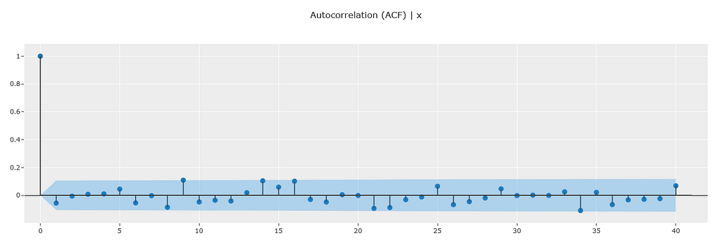
The ACF data shows no significant auto correlations and is consistent with white noise. This is again as expected (see previous reads for details).
👉 Step 3: Theoretical Calculations
Next, let’s get some data statistics from the experiment and add the theoretical calculation from our framework above.
Note: The training and the testing data splits can be obtained using the “get_config” method of the experiment object as shown below.
# Get Train Data
y_train = exp.get_config("y_train")
# Get Test Data
y_test = exp.get_config("y_test")
#########################################################
# Convert into dataframe & add residual calculations ----
#########################################################
train_data = pd.DataFrame({"y":y_train})
train_data['preds'] = y_train.mean()
train_data['split'] = "Train"
test_data = pd.DataFrame({'y': y_test})
test_data['preds'] = y_train.mean()
test_data['split'] = "Test"
data = pd.concat([train_data, test_data])
data['residuals'] = data['y'] - data['preds']
data.reset_index(inplace=True)
Next, let’s compute the calculations needed to make the theoretical prediction and compute the prediction intervals.
#######################################################
#### Compute values based on theoretical equations ----
#######################################################
y_train_mean = data.query("split=='Train'")['y'].mean()
resid_std = data.query("split=='Train'")['residuals'].std(ddof=0)
resid_var = resid_std**2
print(f"Mean of Training Data: {y_train_mean}")
print(f"Std Dev of Residuals: {resid_std}")
print(f"Variance of Residuals: {resid_var}")
>>> Mean of Training Data: 176.01810663414085
>>> Std Dev of Residuals: 0.9884112461876059
>>> Variance of Residuals: 0.976956791590136
######################################
#### Compute Prediction Intervals ----
######################################
import scipy.stats as st
alpha = 0.05
# 2 sided multiplier
multiplier = st.norm.ppf(1-alpha/2)
lower_interval = np.round(y_train_mean - multiplier * resid_std, 2)
upper_interval = np.round(y_train_mean + multiplier * resid_std, 2)
print(f"Prediction Interval: {lower_interval} - {upper_interval}")
>>> Prediction Interval: 174.08 - 177.96
👉Step 4: Build the Model
Now that we have the theoretical calculations out of the way, let’s build this model using PyCaret and check the results. Model creation is as simple as calling the create_model method from the experiment object. Also, you can also pass specific hyperparameters to the model at this time. In our case, we are modeling data without any auto regressive properties, so we will pass all zeros for order and for seasonal_order . If you would like to know more about how to create time series models with PyCaret and how to customize them, please refer to [3].
model1 = exp.create_model(
    "arima",
    order=(0, 0, 0),
    seasonal_order=(0, 0, 0, 0)
)
👉Step 5: Analyze the Results
Next, I have written a few small wrapper functions using PyCaret one-liners to help with model evaluation (see appendix for definition). These are
(1) summarize_model : Produces a statistical summary of the model
(2) get_residual_properties : Plots and displays variance of residuals
(3) plot_predictions : Plots both out-of-sample and in-sample predictions
If you would like to know more about how what these functions are doing, especially the summarize_model, please refer to [4].
Now, let see what we get when we run the model through these helper functions
summarize_model(model1)
get_residual_properties(model1)
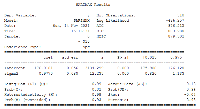

The statistical summary of the model is displayed above. The intercept is the mean of the training data. It matches up with the calculations from our theoretical framework above!
The sigma2 is the variance of the residuals. How do we know? Check the output of the get_residual_properties function. It shows the variance of the residuals. This value matches up exactly with the statistical summary and also with the calculations from our theoretical framework!
But what about the predictions? Let’s check that next.
plot_predictions(model1)
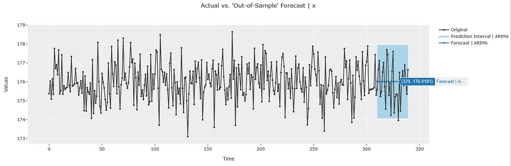
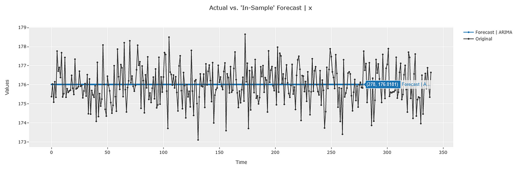
PyCaret by default provides interactive plots using the plotly library so we can quickly verify the values by hovering over the plot. We can quickly see that both the out-of-sample and in-sample predictions are equal to 176.02 which matches the calculations from our theoretical framework. The prediction interval also matches the values from our theoretical framework!
🚀 Conclusion
Hopefully this simple model has laid a good foundation for us to understand the inner workings of an ARIMA model. In the next set of articles, we will start covering the other parameters one by one and see the impact that they have on the model’s behavior. Until then, if you would like to connect with me on my social channels (I post about Time Series Analysis frequently), you can find me below. That’s it for now. Happy forecasting!
📘 GitHub
📗 Resources
- Jupyter Notebook containing the code for this article
📚 References
[1] Diagnosing “White Noise” in PyCaret
[2] Modeling “White Noise” in PyCaret
[3] Creating and Customizing a Time Series Model
[4] Understanding the underlying architecture of the PyCaret Time Series Module
[5] Chapter 8 ARIMA Models, Forecasting: Principles and Practice, Rob J Hyndman and George Athanasopoulos
📘 Appendix
- Helper Functions
def summarize_model(model):
    """
    Provides statistical summary for some statistical models
    """
    # Statistical Summary Table
    try:
        print(model.summary())
    except:
        print("Summary does not exist for this model.")
def get_residual_properties(model):
    """
    Plots and displays variance of residuals
    """
    #### Residuals ----
    try:
        plot_data = exp.plot_model(
            model,
            plot="residuals",
            return_data=True
        )
        residuals = plot_data['data']
        residuals_var = residuals.std(ddof=0)**2
        print(f"Variance of Residuals: {residuals_var}")
    except:
        print("Residuals can not be extracted for this model.")
def plot_predictions(model):
    """
    Plots out-of-sample and in-sample predictions
    """
    # Out-of-Sample Forecast
    exp.plot_model(model)
# In-Sample Forecast
    exp.plot_model(model, plot="insample")
Understanding ARIMA Models using PyCaret’s Time Series Module — Part 1 was originally published in Towards Data Science on Medium, where people are continuing the conversation by highlighting and responding to this story.
from Towards Data Science - Medium https://ift.tt/3FylhJe
via RiYo Analytics


No comments