https://ift.tt/3oiw5EA A Gradient Boosted Time-Series Decomposition Method Photo by Allan Swart on iStock TLDR: ThymeBoost combines ...
A Gradient Boosted Time-Series Decomposition Method

TLDR: ThymeBoost combines the traditional decomposition process with gradient boosting to provide a flexible mix-and-match time series framework for trend/seasonality/exogenous decomposition and forecasting, all a pip away.
All code lives here: ThymeBoost Github
A Motivating Example
Traditional time-series decomposition typically involves a sequence of steps:
- Approximate Trend/Level
- Detrend to Approximate Seasonality
- Detrend and Deseasonalize to Approximate Other Factors (Exogenous)
- Add Trend, Seasonality, and Exogenous for the results
Depending on certain algorithms at each step we may need to switch up the order and deseasonalize first. Either way, at first glance we can convince ourselves that this process flow is…fine.
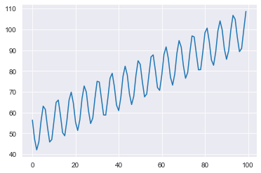
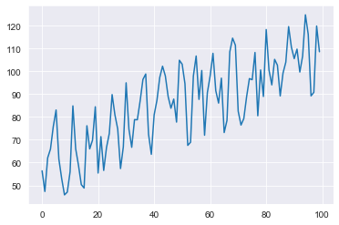
In fact, it can do quite well in a simple simulation. Let’s make a basic trend + seasonality time-series to show how the process works.
import numpy as np
import matplotlib.pyplot as plt
import seaborn as sns
sns.set_style("darkgrid")
#Here we will just create a simple series
np.random.seed(100)
trend = np.linspace(1, 50, 100) + 50
seasonality = ((np.cos(np.arange(1, 101))*10))
y = trend + seasonality
#let's plot it
plt.plot(y)
plt.show()
And now to do some basic decomposition.
Following the above process, we will first fit a simple linear trend to approximate the trend component:
import statsmodels.api as sm
#A simple input matrix for a deterministic trend component
X = np.array([range(1, len(y) + 1),
              np.ones(len(y))]).T
mod = sm.OLS(y, X)
res = mod.fit()
fitted_trend = res.predict(X)
plt.plot(trend)
plt.plot(fitted_trend, linestyle='dashed')
plt.show()
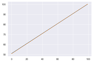
That trend line is spot on! We will subtract the fitted trend from our actuals and use that detrended signal to approximate the seasonal component:
detrended_series = y - fitted_trend
#Set the seasonal period
seasonal_period = 25
#Get the average of every 25 data points to use as seasonality
avg_season = [np.mean(detrended_series[i::seasonal_period], axis=0) for i in range(seasonal_period)]
avg_season = np.array(avg_season)
fitted_seasonality = np.resize(avg_season, len(y))
plt.plot(fitted_seasonality)
plt.plot(seasonality)
plt.show()
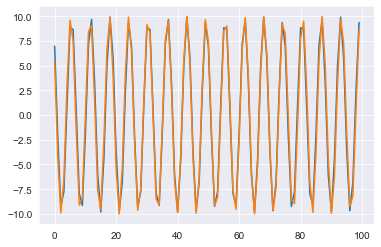
That seasonal component looks good as well! While we see slight deviations, overall the two lines are almost identical. You may have noticed that there is no legend in the plots. This is because our signal has no noise by design, so the decomposition and the series are essentially the same. The decomposition process is quite well behaved, not necessitating a legend…yet.
Let’s put it all together and see our full results:
fitted = fitted_trend + fitted_seasonality
plt.plot(fitted, linestyle='dashed')
plt.plot(y, linestyle='dashed')
plt.show()
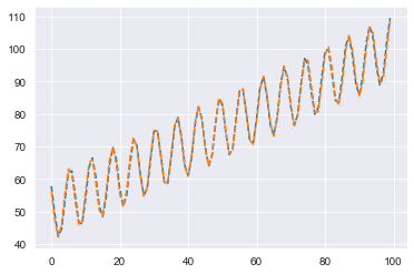
The final results for the decomposition are quite compelling. This process gives us complete control over the different components. Let’s say we needed to treat seasonality differently than the trend, possibly by giving certain samples more or less weight:
We can.
Additionally, if we add an exogenous factor we could approximate that component with any model we want. If we have plenty of data and complicated features we could simply subtract out the trend and seasonal component, then feed those residuals to XGBoost.
But for this example, let’s add a simple ‘holiday’ effect to our current series and fit that with a linear regression. First, we will rebuild our simulated series but now adding in that exogenous factor.
np.random.seed(100)
trend = np.linspace(1, 50, 100) + 50
seasonality = ((np.cos(np.arange(1, 101))*10))
exogenous = np.random.randint(low=0, high=2, size=len(trend))
y = trend + seasonality + exogenous * 20
plt.plot(y)
plt.show()
We simply created a random series of 1’s and 0’s as our ‘exogenous’ and gave it an effect of adding 20 to our series when 1. Now if we repeat the same process as before we will notice that it doesn’t hold up quite as well.
import statsmodels.api as sm
#A simple input matrix for a deterministic trend component
X = np.array([range(1, len(y) + 1),
              np.ones(len(y))]).T
mod = sm.OLS(y, X)
res = mod.fit()
fitted_trend = res.predict(X)
plt.plot(trend, label='actual trend')
plt.plot(fitted_trend, linestyle='dashed', label='fitted trend')
plt.legend()
plt.show()
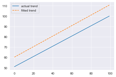
Clearly that trend is off. We do approximate the correct slope but we have an incorrect intercept. This is quite concerning because we feed the detrended series to approximate the seasonality, further compounding the error. Additionally, we do not allow any adjustments for the trend.
We have one shot to get it right.
Either way, let’s move on to approximating the seasonal component:
#Set the seasonal period
seasonal_period = 25
#Get the average of every 25 data points to use as seasonality
avg_season = [np.mean(detrended_series[i::seasonal_period], axis=0) for i in range(seasonal_period)]
avg_season = np.array(avg_season)
fitted_seasonality = np.resize(avg_season, len(y))
plt.plot(fitted_seasonality, label='fitted seasonality')
plt.plot(seasonality, label='actual seasonality')
plt.legend()
plt.show()
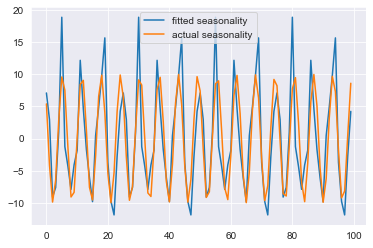
As expected, the seasonal component is not only negatively affected by the incorrect trend, it also appears to be eating up the signal from the exogenous factor. Let’s see if this is the case by plotting the residuals:
residuals = y - fitted_trend - fitted_seasonality
plt.plot(residuals)
plt.show()
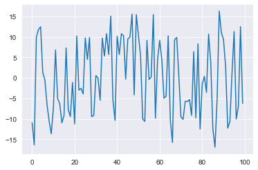
Recall that the exogenous factor simply added 20 when equal to 1. In a perfect world these residuals should be random noise around 0 along with spikes of 20. Without this, it is doubtful that our exogenous approximation will be correct, but let’s try it out anyway.
To approximate the exogenous component we will fit with the residuals from detrending and deseasonalizing.
X = np.column_stack([exogenous, np.ones(len(y))])
mod = sm.OLS(residuals, X)
res = mod.fit()
print(res.summary())
Let’s take a look at the summary from OLS:
"""
                            OLS Regression Results
==============================================================================
Dep. Variable:                      y   R-squared:           0.768
Model:                            OLS   Adj. R-squared:      0.766
Method:                 Least Squares   F-statistic:         325.1
Date:                Wed, 10 Nov 2021   Prob (F-statistic): 6.82e-33
Time:                        09:46:43   Log-Likelihood:     -289.29
No. Observations:                 100   AIC:                 582.6
Df Residuals:                      98   BIC:                 587.8
Df Model:                           1
Covariance Type:            nonrobust
==============================================================================
                 coef    std err          t      P>|t|
------------------------------------------------------------------------------
x1            15.9072      0.882     18.032      0.000          17.658
const         -7.9536      0.624    -12.750      0.000
====================================================================
The expected impact of our exogenous factor has been shrunken from 20 to 16! Based on everything we have seen up to this point, this should not be a surprise. Any slight mistake early on in the process creates compounding errors later and there is no mechanism for adjustments.
Putting everything together:
fitted_exogenous = res.predict(X)
fitted = fitted_trend + fitted_seasonality + fitted_exogenous
plt.plot(y, label='actuals')
plt.plot(fitted, label='fitted')
plt.legend()
plt.show()
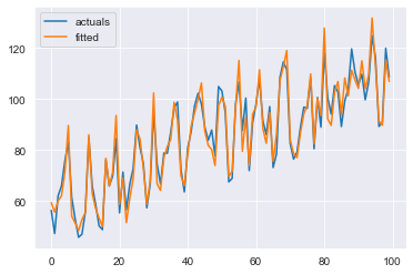
Given everything that went wrong during this process, this result looks ok. Remember this is a simulated ‘pristine’ time-series, so the fact that we were able to break the process quite easily should be concerning. It seems that the process may be too rigid. Since the seasonal component eats up some signal of the exogenous component, should we switch the order of approximation? What if our trend is more complicated and we have to use a more complex method such as Double-Exponential Smoothing? Wouldn’t that also potentially eat the seasonality signal AND exogenous signal?
We can simply fix this issue by NOT doing this process at all. We can move to a method which approximates all components at once such as Facebook’s Prophet model or possibly some other GAM-like setup. But that comes at the cost of losing some control over the individual components. We no longer can fit different components with different methods; the process has been simplified but so have our potential forecasts.
The question is:
How can we obtain the benefits of a single fitting procedure, but retain full control over our individual components?
The answer is:
Apply Gradient Boosting to our Time-Series Decomposition.
A Natural Next Step
A simple adjustment to the previous process flow will aid us in emulating a simultaneous fitting procedure. After we approximate the last step we will use the residuals and refit the whole procedure.
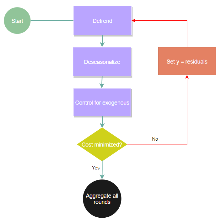
This boosting continues until some global cost function is minimized. Furthermore, we can utilize even more concepts found in gradient boosting, such as a learning rate. But now we can apply a learning rate to each individual component, alleviating any issues of the seasonality eating up exogenous signals. Additionally, we can allow the trend component to search for changepoints via binary segmentation and, through boosting, end up with a very complicated model. The complexity that can now be achieved by simply boosting is bonkers (I believe that is the technical word for it). This newly achieved complexity leads to more shapes we can forecast, meaning higher potential for better accuracy. We can quickly build an ARIMA with 5 changepoints, seasonality approximated via Fourier basis functions, and boosted trees for exogenous forecasting.
But first, let’s just forecast our simple series.
ThymeBoost
ThymeBoost is a dev package for Python and it contains all of the functionality laid out so far (and more). But a word of warning before continuing, it is still in early development so one could encounter bugs. Please use at your own risk. I recommend going through the README examples on GitHub as well as following along here.
First, let’s install from pip, you will definitely want the most up-to-date statsmodels and sci-kit learn packages:
pip install ThymeBoost
Next let’s rebuild our simulated series here:
import numpy as np
import matplotlib.pyplot as plt
import seaborn as sns
sns.set_style('darkgrid')
np.random.seed(100)
trend = np.linspace(1, 50, 100) + 50
seasonality = ((np.cos(np.arange(1, 101))*10))
exogenous = np.random.randint(low=0, high=2, size=len(trend))
y = trend + seasonality + exogenous * 20
Import ThymeBoost and build the class:
from ThymeBoost import ThymeBoost as tb
boosted_model = tb.ThymeBoost(verbose=1)
The verbose argument simply denotes whether to print logs of the boosting process. All that is left to do is to fit our series exactly as before, but this time with some added ThymeBoost magic.
output = boosted_model.fit(y,
                           trend_estimator='linear',
                           seasonal_estimator='classic',
                           exogenous_estimator='ols',
                           seasonal_period=25,
                           global_cost='maicc',
                           fit_type='global',
                           exogenous=exogenous)
First, let’s walkthrough some of these arguments:
trend_estimator: How you want to approximate the trend, here ‘linear’ is a simple regression as before.
seasonal_estimator: I’m sure you guessed it, the method to approximate seasonality, ‘classic’ uses a simple average of every seasonal_period.
exogenous_estimator: The method used to calculate the exogenous component.
seasonal_period: The expected seasonal period.
global_cost: Finally, an interesting argument! This controls the boosting procedure, ‘maicc’ is a ‘modified Akaike-Information Criterion’ where the modifications are used to incorporate boosting rounds into the formulation.
fit_type: Here we denote whether we want ThymeBoost to look for changepoints or not, ‘global’ will fit our trend_estimator to all data. If we pass ‘local’ then we will do binary segmentation to find a potential changepoint.
The results saved to ‘output’ is a Pandas DataFrame with the fitted values and each individual component. If you have experience with Prophet then this should remind you of that.
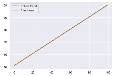
Let’s plot the fitted trend, seasonality, and exogenous component and see how it did.
Approximated Trend:
plt.plot(trend, label='actual trend')
plt.plot(output['trend'], label='fitted trend')
plt.legend()
plt.show()
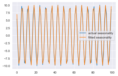
Approximated Seasonality:
plt.plot(seasonality, label='actual seasonality')
plt.plot(output['seasonality'], label='fitted seasonality')
plt.legend()
plt.show()
Approximated Exogenous
plt.plot(exogenous * 20, label='actual exogenous')
plt.plot(output['exogenous'], label='fitted exogenous')
plt.legend()
plt.show()
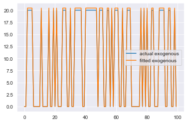
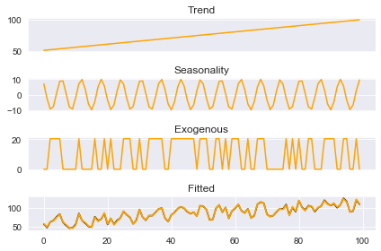
This is quite an improvement over the traditional process. We were able to accurately approximate each individual component. ThymeBoost also provides some helper functions for quicker plotting:
boosted_model.plot_components(output)
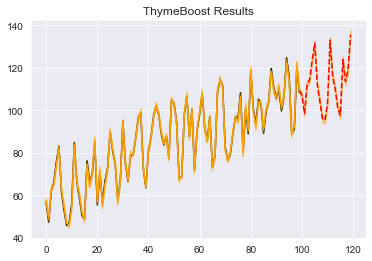
The package utilizes the standard fit-predict methods. Let’s use ThymeBoost to create predictions and plot them using the plot_results method :
#create a future exogenous input
forecast_horizon = 20
np.random.seed(100)
future_exogenous = np.random.randint(low=0, high=2, size=forecast_horizon)
#use predict method and pass fitted output, forecast horizon, and future exogenous
predicted_output = boosted_model.predict(output,
                                         forecast_horizon=forecast_horizon,
                                         future_exogenous=future_exogenous)
boosted_model.plot_results(output, predicted_output)
Conclusion
ThymeBoost fixes many of the major issues with traditional time-series decomposition and allows us to retain complete control over each component. The procedure even gives us access to interesting new features due to the boosting iterations. For example, a common issue in time-series is multiple seasonality. Thymeboost can solve this quite naturally by changing the seasonal period during each boosting round, with a simple change to our fit call, now passing a list to seasonal_period.
From:
output = boosted_model.fit(y,
                           trend_estimator='linear',
                           seasonal_estimator='classic',
                           exogenous_estimator='ols',
                           seasonal_period=25,
                           global_cost='maicc',
                           fit_type='global',
                           exogenous=exogenous)
To:
output = boosted_model.fit(y,
                           trend_estimator='linear',
                           seasonal_estimator='classic',
                           exogenous_estimator='ols',
                           seasonal_period=[25, 5],
                           global_cost='maicc',
                           fit_type='global',
                           exogenous=exogenous)
ThymeBoost will go back and forth between the two seasonal periods provided in the list, making adjustments to the total seasonal component each time. But it doesn’t stop at seasonality. We can also do this with every argument passed to fit. Meaning we can start with a simple linear trend followed by ARIMA and then Double-Exponential Smoothing in the final boosting round. You have complete control over the entire procedure.
As mentioned before, this package is still in early development. The sheer number of possible configurations makes debugging an involved procedure, so use at your own risk. But please, play around and open any issues you encounter on GitHub!
Time Series Forecasting with ThymeBoost was originally published in Towards Data Science on Medium, where people are continuing the conversation by highlighting and responding to this story.
from Towards Data Science - Medium https://ift.tt/3c03UVb
via RiYo Analytics


ليست هناك تعليقات