https://ift.tt/3nNbWGb A TCN Tutorial, Using the Darts Multi-Method Forecast Library Yesterday’s article offered a tutorial on recurrent n...
A TCN Tutorial, Using the Darts Multi-Method Forecast Library
Yesterday’s article offered a tutorial on recurrent neural networks (RNNs): their LSTM, GRU, and Vanilla variants. Today, let’s add Temporal Convolutional Networks (TCNs), as the tenth method in the fourth article of this little series on time series forecasters.

- Temporal Loops: Intro to Recurrent Neural Networks for Time Series Forecasting in Python | Towards Data Science
- Wisdom of the Forecaster Crowd. Ensemble Forecasts of Time Series in Python | Towards Data Science
- Darts’ Swiss Knife for Time Series Forecasting | Towards Data Science
The RNN tutorial offered a quick run-down of neural networks in general and recurrent neural networks in particular by describing their core features and terminology. Today’s article will start from this basis and then highlight the aspects in which temporal convolutional networks differ from RNNs.
We will build a TCN by using the Darts library, which wraps the neural networks available in the PyTorch package; and then run our TCN in a small tournament against the three RNN variants and the Theta method we encountered yesterday.
1. Concept of Temporal Convolutional Networks (TCNs)
Convolutional neural networks (CNNs) are commonly applied to computer vision tasks: image or video recognition and classification.

A 2018 article by Sumit Saha gives an excellent overview for the use of CNNs in image processing (A Comprehensive Guide to Convolutional Neural Networks — the ELI5 way | by Sumit Saha | Towards Data Science).
The basic architecture of a convolutional neural network was first proposed in 1979, inspired by earlier studies of the visual cortex. The resulting “neocognitron” was applied to the recognition of handwritten Japanese characters.
The core architecture of a CNN consists of an input layer, hidden layers, among them the convolutional layer, and the output layer. The hidden layers perform the convolutions. Pooling layers collect and consolidate the intermediate results. Fully connected layers attempt to derive a nonlinear function that describes the mapping of the input values to the outputs. The TCN, similar to RNNs, also has a cost or loss function which it seeks to minimize to reduce the prediction error.
A convolution is an operation in integral calculus. The convolution takes two functions, one of which is reversed and shifted, and calculates the integral of their product. The convolution function expresses how the shape of one function is modified by the other. The convolution resembles cross-correlation in that it reflects the similarity of two series or sequences.
The inputs a given node oversees, leaning on computer vision terminology, are called a receptive field or a patch. Each node receives inputs from a limited patch of the network’s previous layer, the node’s receptive field.
CNNs apply filters to the input to detect the presence of a feature. Its nodes or neurons act as these filters.
In an image, a shape or color can represent a feature. A filter can specialize, for instance, on the detection of vertical lines. Other filters will hook themselves up to other features, for instance horizontal lines. In a time series, the trend or seasonality are features to be isolated. The values of the filters are the weights the CNN will calibrate during training to minimize the prediction error expressed in the loss function. When classifying images in a search for pictured pets, the CNN will learn to isolate the characteristic features of dogs or cats and thus build a dogginess or cattiness classifier with the help of the filters it has trained. When dealing with time series, it can learn to recognize their trend and seasonality patterns.
The nodes create a feature map, mapping out the presence of a feature. A filter moves across its patch of inputs and checks it for the presence of the feature. The results get collected in the feature map. The kernel or feature detector is a two-dimensional array of weights. The kernel moves across the receptive fields of an image to detect the feature. The distance the filter moves across the input is referred to as the stride.
Fully connected layers receive the extracted features as their inputs and apply an activation function. This layer gets its name because it connects every node in one layer to every node in another layer: the receptive field of a node in a fully connected layer is the entire previous layer. The fully connected layer builds a usually nonlinear function that ties together the features it receives from the previous layers.
The CNN paces through a sequence of training epochs — feed-forward followed by backpropagation — and learns to sort out unimportant features from the essential ones.
Temporal convolutional networks — a recent development (An Empirical Evaluation of Generic Convolutional and Recurrent Networks for Sequence Modeling (arxiv.org)) — add certain properties of recurrent neural networks to the classic CNN design.
The TCN ensures causal convolution. An output value must only depend on values that are positioned earlier in the input sequence.
Dilations in the TCN expand the receptive field of a node to encompass more historical periods.
2. Dependencies
From among the Darts models, we now also import the TCNModel subclass in line 8.
We make a small change to yesterday’s RNN-related script by experimenting with a dropout level different from zero, 0.1, both for the three RNNs and the TCN. Dropout level denotes an option which switches nodes in the network on or off. This is to prevent overfitting. The nodes are less prone to dig themselves deeper and deeper into a particular configuration of connected nodes. Convolutional networks have a higher propensity for overfitting, therefore we don’t leave the dropout level switched off.
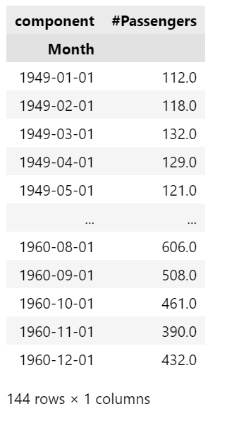
Darts integrates some of the classic data sources, among them Box & Jenkins’ airline passenger dataset, which we can load from the library without needing to import a file.
In the airline passenger example, I choose August 1, 1958 for the start of the test period, expressed in the constant FC_START. We are going to forecast 12 months, entered in constant FC_N.
3. Preparing the Data
Darts’ load() function allows us to read the time series into a timeseries object.
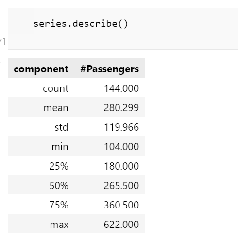
The function pd_dataframe() can convert the timeseries object to “normal” series and to a dataframe to make it compatible with the methods pandas offers for data wrangling.
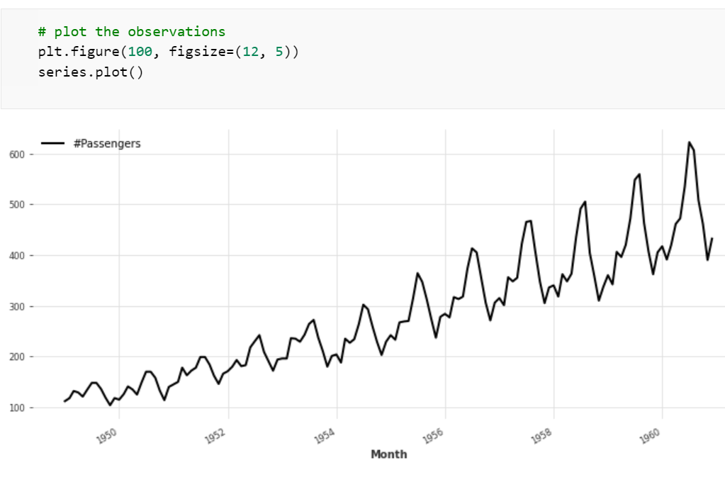
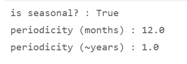
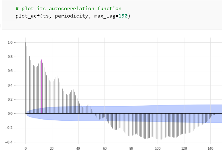
The chart reveals a seasonality that closely resembles that of 12 months in a calendar year. To confirm, we apply Darts’ check_seasonality() test, which evaluates the autocorrelation function ACF. The test confirms that the periodicity of the time series is precisely 12.0 months. This suggests, like the chart did, a time series with a comparatively simple pattern.
Next, we split the time series into a training and a validation dataset at the time period FC_START we’ve chosen as a constant in the dependencies cell: 19580801.
Before feeding the source data into neural networks, we need to normalize them by applying a Scaler() function. Normalization counteracts the exploding gradient problem the previous article has mentioned. The scaling will also make it easier for the neural network to run the gradient descent in search for a minimal prediction error.
At present, the time series’ dates are encoded in strings. To enable the TCN to recognize the time steps, we extract from these strings the months and define them as a second column — a covariate or exogenous regressor — by applying Darts’ datetime_attribute_timeseries() function. Then we normalize the covariate with a scaler.
4. Setup of the Model
The list models lines up the four neural networks we want to let loose on the time series: the TCN model we are introducing today; and the three flavors of recurrent neural networks we had devised in yesterday’s tutorial: LSTM, GRU, and Vanilla RNN.
In row 5, we prepare a conditional list comprehension that will read the four models one after the other and pass them to the setup functions we will write below.
Note the ‘if — else’ condition in the list comprehension. The parameter setups of TCN and RNN are different, therefore the list comprehension calls different functions — run_TCN() and run_RNN() — for them. It will collect their results — the prediction accuracy metrics — in the variable res_models.
The training function for the RNN models, run_RNN(), is basically the same as we had discussed in yesterday’s article. I will skip the RNNs parts and focus on the TCN.
The function run_TCN() has a similar shape, but differs in some aspects from that of the RNNs.
We set the input_chunk_length — the number of past periods to be used for predictions — to 13 months, 1 more month than the periodicity the check_seasonality test has returned. The RNN will look back 13 months in the past, a full seasonal cycle, to compute predictions.
The output_chunk_length we choose comprises the 12 months of a full seasonal cycle. It must be strictly smaller than the input_chunk_length, therefore the 13 months for the input. The forecast horizon is limited to the output length.
To experiment, we set the dropout level to 0.1 instead of the zero rate we used previously. The dropout level will help to simulate different network architectures. At every epoch, the network selects a different set of neurons which it temporarily removes. Different combinations of neurons then make the predictions. These recombinations will prevent the TCN from overfitting to the same set of neurons.
The number of filters should reflect the supposed intricacy of the patterns inherent in the time series. The visual clues we’ve got from the line chart suggest a relatively simple time series, with a trend and a single order of seasonality. Therefore, three to five filters should be more than enough to mirror its complexity.
The Boolean parameter weight_norm determines whether or not the TCN will use weight normalization. Normalization has the effect that the length of the weight vectors is decoupled from their direction, which will speed up the gradient descent towards the minimal error (Weight Normalization: A Simple Reparameterization to Accelerate Training of Deep Neural Networks (neurips.cc)). Yet a study finds that an alternative approach, batch normalization, may result in better test accuracy ([1709.08145] Comparison of Batch Normalization and Weight Normalization Algorithms for the Large-scale Image Classification (arxiv.org)). Therefore, weight norm is a hyperparameter the user can choose to tweak.
The dilation base factor makes the TCN reach out to nodes that are farther back in time. This expands the receptive field of a node to encompass more historical periods. It provides the TCN with memory. The kernel size should be set at least as large as the chosen dilation factor.
After the setup of the model in lines 6 to 18, we fit it to the training data in lines 23 to 28. The fitter refers to both the training and the validation dataset and uses both their time series values and the series of months we defined as the covariates.
Lines 35 to 37 derive the 12 months of predicted values.
In line 40, we call the same plotter function, plot_fitted(), as for the RNN models.
Line 43 feeds the predictions and the actual values to the accuracy_metrics() function, which will compute the mean absolute percentage error and some other prediction quality indicators.
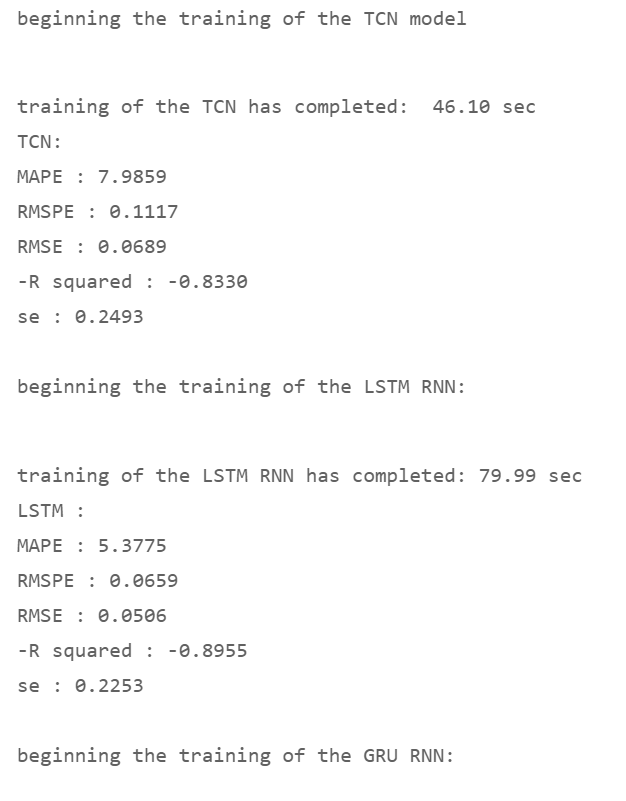
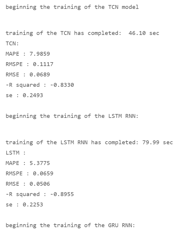
While the script is fitting the four models, it displays its progress and then reports the resulting accuracy metrics:

The plotter function draws the actual observations and the 12 months of predictions. The lines of the blue forecast values are hugging the black actual curve relative closely.
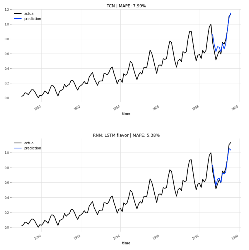
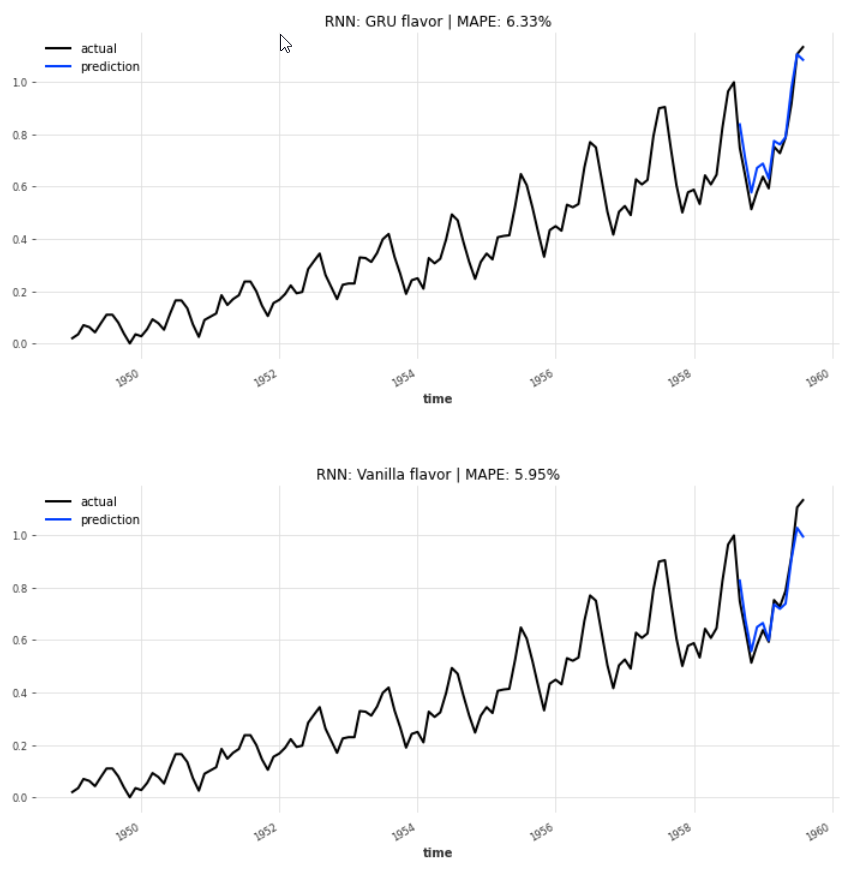
The LSTM variant of recurrent neural networks boasts the lowest MAPE, at 5.38% , followed by the Vanilla flavor at 5.95%. The TCN could not play out its strengths in this example and reports a distinctively higher MAPE, 7.99%, than the three RNNs.
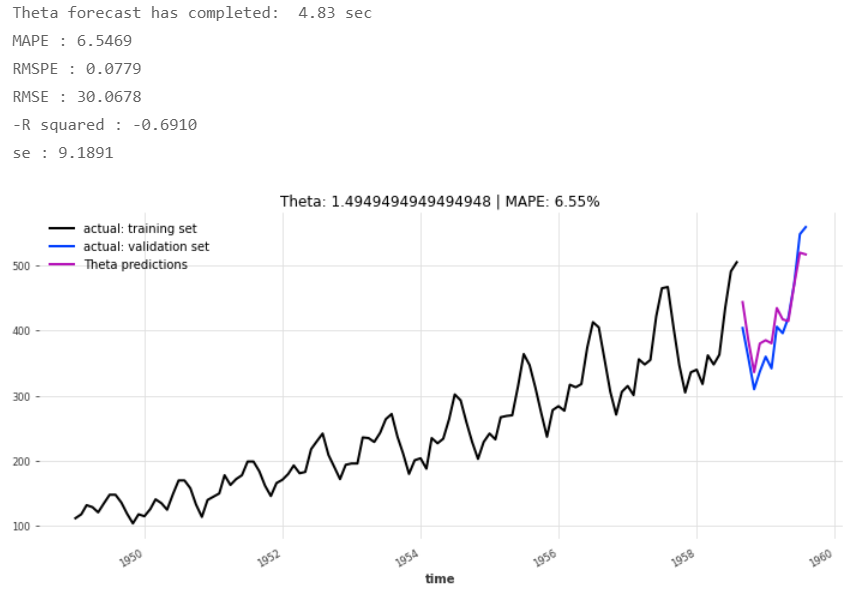
As we did yesterday, we prepare a quick baseline forecast by applying a non-neural network forecaster, the Theta method, which will run it seconds, and compare this benchmark with the TCN and the RNNs.
5. Conclusions
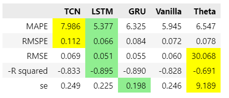
The Theta forecast’s prediction errors rank it behind all three RNN flavors, though it has a lower MAPE and root mean squared percentage error RMSPE than the TCN has achieved.
The absolute RMSE and the R-squared — the share of the movements in the predictions that are aligned with the movements in the actual observations — are better for the TCN than for Theta in this example. But the three RNNs still outcompete both TCN and Theta.
This particular example did not suit the TCN well, but studies of times series problems with more complex patterns — for instance the prediction of the El Niño-Southern Oscillation, the cyclical, non-seasonal warming of the Pacific Ocean’s surface — found a TCN accuracy that was superior to that of recurrent neural networks (Temporal Convolutional Networks for the Advance Prediction of ENSO |(nature.com)).
The Jupyter notebook is available for download on GitHub: h3ik0th/Darts_TCN_RNN: time series forecasting with TCN and RNN neural networks in Darts (github.com)
Temporal Coils: Intro to Temporal Convolutional Networks for Time Series Forecasting in Python was originally published in Towards Data Science on Medium, where people are continuing the conversation by highlighting and responding to this story.
from Towards Data Science - Medium https://ift.tt/3mzQkOn
via RiYo Analytics


No comments