https://ift.tt/3r2NB2s Review of the seminal paper and implementations to uncover the best option for your data Photo by Алекс Арцибашев ...
Review of the seminal paper and implementations to uncover the best option for your data

Comparing prediction methods to define which one should be used for the task at hand is a daily activity for most data scientists. Usually, one will have a pool of classification models and will validate them using cross-validation to define which one is best.
Another goal, however, is not to compare classifiers, but the learning algorithms themselves. The idea is: given this task (data), which learning algorithm (KNN, SVM, Random Forests, etc) will generate more accurate classifiers on a dataset of size D?
As we will see, every method presented here has some pros and cons. However, the first intuition of using a two proportions test can lead to some really bad results.
To learn more about how we can compare these algorithms and also improve our knowledge of Statistics, today I will be explaining and implementing the methods from the Approximate Statistical Tests for Comparing Supervised Classification Learning Algorithms [1], a seminal paper on this area.
In the next sections, I will describe each of the tests, talk about its strengths and weaknesses, implement them and then compare the results with an available implementation.
The notebook for this post is available on Kaggle and also on my Github.
Initial Code Setup
For the codes in this post, we will be using two classification algorithms: a KNN and a Random Forest to predict wine quality on the Wine dataset [2] from the UCI Machine Learning Repository that is freely available on the sklearn package. To do so, we will import some required libraries and will instantiate the algorithms:
# Importing the required libs
import numpy as np
import pandas as pd

from tqdm import tqdm
from scipy.stats import norm, chi2
from scipy.stats import t as t_dist
from sklearn.datasets import load_wine
from sklearn.metrics import accuracy_score
from sklearn.ensemble import RandomForestClassifier
from sklearn.neighbors import KNeighborsClassifier
from sklearn.model_selection import train_test_split, KFold

# Libs implementations
from mlxtend.evaluate import mcnemar
from mlxtend.evaluate import mcnemar_table
from mlxtend.evaluate import paired_ttest_5x2cv
from mlxtend.evaluate import proportion_difference
from mlxtend.evaluate import paired_ttest_kfold_cv
from mlxtend.evaluate import paired_ttest_resampled
# Getting the wine data from sklearn
X, y = load_wine(return_X_y = True)
# Instantiating the classification algorithms
rf = RandomForestClassifier(random_state=42)
knn = KNeighborsClassifier(n_neighbors=1)
# For holdout cases
X_train, X_test, y_train, y_test = train_test_split(X, y, test_size=0.20, random_state=42)
Two Proportions Test
Comparing two proportions is a very old problem and statistics have a classical hypothesis test to solve it: given two proportions from two populations, the null hypothesis is that the difference between the proportions has a mean equal to zero.
One can calculate this with the following statistic:

Seems pretty simple, right? We just get the proportion of hits of our algorithms (accuracy) and compare it. However, there is one important assumption on this test: the independence of samples.
As one can quickly guess, the samples here are not independent since the test and train sets are the same for both algorithms. So this assumption goes south.
There are other two problems with this approach:
- It does not take into account the variance of the test set. If we change it we may have very different results
- It does not account for the entire dataset, rather, it accounts for a smaller set of it that was selected to be used on training
To use this test, one can use the following code:
# First we fit the classification algorithms
rf.fit(X_train, y_train)
knn.fit(X_train, y_train)
# Generate the predictions
rf_y = rf.predict(X_test)
knn_y = knn.predict(X_test)
# Calculate the accuracy
acc1 = accuracy_score(y_test, rf_y)
acc2 = accuracy_score(y_test, knn_y)
# Run the test
print("Proportions Z-Test")
z, p = proportion_difference(acc1, acc2, n_1=len(y_test))
print(f"z statistic: {z}, p-value: {p}\n")
Here we are simply fitting the algorithms on the hold-out test set and running the test on the resulting accuracies.
Resampled Paired t-test
To account for the variance of the test set, one can use the Resampled Paired t-test. In this test, we will set a number of trials (e. g 30) and will measure the accuracy of each algorithm on each trial using a holdout test set.
Then, if we assume that p_i = pA_i - pB_i, for every trial i is normally distributed, we can apply the paired Student’s t-test:

Because on each trial we change our test set, its variance is taken into account, improving on one of the problems of the previous test. However, we still have some problems in our hands:
- The normal distribution for p_i does not hold because the proportions are not independent since they are calculated on the same test set
- There is overlap between the training sets and the test sets on each of the trials, so the p_i’s are not independent
- It requires our algorithms to be fitted many times, which may be prohibitive if the fitting time is too long
For this implementation, we will define create a function that will receive the p_is as a parameter:
def paired_t_test(p):
    p_hat = np.mean(p)
    n = len(p)
    den = np.sqrt(sum([(diff - p_hat)**2 for diff in p]) / (n - 1))
    t = (p_hat * (n**(1/2))) / den

    p_value = t_dist.sf(t, n-1)*2

    return t, p_value
On this function, we are just creating the t statistic from the test following the equation. Then, we use a Student’s t distribution from scipy to find out the p-value for the test and we then return the statistic and the p-value.
The code to run the resampled t-test goes as follows:
n_tests = 30

p_ = []
rng = np.random.RandomState(42)
for i in range(n_tests):
    randint = rng.randint(low=0, high=32767)
    X_train, X_test, y_train, y_test = train_test_split(X, y, test_size=0.20, random_state=randint)
    rf.fit(X_train, y_train)
    knn.fit(X_train, y_train)

    acc1 = accuracy_score(y_test, rf.predict(X_test))
    acc2 = accuracy_score(y_test, knn.predict(X_test))
    p_.append(acc1 - acc2)

print("Paired t-test Resampled")
t, p = paired_t_test(p_)
print(f"t statistic: {t}, p-value: {p}\n")
Here we define the number of iterations as 30 and for each one, we split the data, fit the classifiers and then calculate the difference between the accuracies. We save this value on a list and then we call the function we defined above with this list.
The Mlxtend library already has this test implemented, so one can also use:
print("Paired t-test Resampled")
t, p = paired_ttest_resampled(estimator1=rf, estimator2=knn, X=X,y=y, random_seed=42, num_rounds=30, test_size=0.2)
print(f"t statistic: {t}, p-value: {p}\n")
Notice that we must pass the entire training set for the function because it will create the splits inside itself. You can verify that the results are the same given the same seed.
Cross-Validated Paired t-test
This method will have the same structure as the one above. However, instead of using a hold-out test set on each trial, we will run cross-validation with K folds.
This will remove the problem of overlapping tests sets since now every sample will be tested against different data.
However, we still have the overlapping train data problem. On 10-fold cross-validation, each training round shares 80% of the training data with the others.
Also, we still have a time problem because we must fit our classifiers several times. However, usually less than the resampled paired t-test since its usual to run 10-fold or 5-fold cross-validation which is way smaller than the 30 tests we did previously.
For this test we will use the same function we defined on the previous test because it will be a t-test anyway, we just need to change how we divide our data on each iteration of the loop (and of course, the number of iterations on the loop as well). Using the KFold from the sklearn library, we have:
p_ = []

kf = KFold(n_splits=10, shuffle=True, random_state=42)
for train_index, test_index in kf.split(X):
    X_train, X_test, y_train, y_test = X[train_index], X[test_index], y[train_index], y[test_index]
    rf.fit(X_train, y_train)
    knn.fit(X_train, y_train)

    acc1 = accuracy_score(y_test, rf.predict(X_test))
    acc2 = accuracy_score(y_test, knn.predict(X_test))
    p_.append(acc1 - acc2)

print("Cross Validated Paired t-test")
t, p = paired_t_test(p_)
print(f"t statistic: {t}, p-value: {p}\n")
Mlxtend also has an implementation for this test:
t, p = paired_ttest_kfold_cv(estimator1=rf, estimator2=knn, X=X, y=y, random_seed=42, shuffle=True, cv=10)
print(f"t statistic: {t}, p-value: {p}\n"
McNemar’s Test
This test has the advantage of requiring only one fit for each of our algorithms. We use a holdout set to fit each one of them and then we create a contingency table:
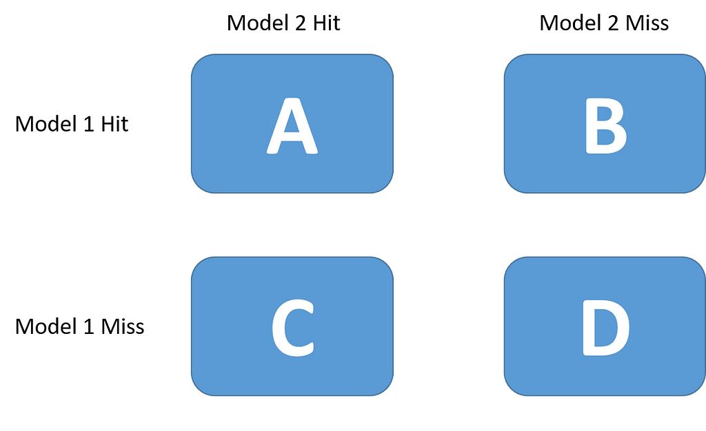
Then, we state the null hypothesis that both algorithms should have the same error rate and do a chi-squared test with the following statistic:

On the paper benchmarks test, this test was classified as the second-best in terms of error rate when compared with the others, losing only to the 5x2 Cross-Validation Test we will see below. Because of that, the authors say that this should be used if you cannot afford cross-validation.
However, there are still problems with this:
- The test does not account for train set variation since we fit only one time
- Because we fit only once, we do not take into account the internal algorithm variation
- We use a smaller set than the original. However, notice that every test here will suffer from that
To implement the test, we will create a dedicated function:
def mcnemar_test(y_true, y_1, y_2):
    b = sum(np.logical_and((knn_y != y_test),(rf_y == y_test)))
    c = sum(np.logical_and((knn_y == y_test),(rf_y != y_test)))

    c_ = (np.abs(b - c) - 1)**2 / (b + c)

    p_value = chi2.sf(c_, 1)
    return c_, p_value
Here we are just calculating the values from the contingency table, seeing where the models have the correct or incorrect answers. Then, we look at the chi-squared distribution to find the p-value for the statistics we calculated.
As this uses a holdout set, the following steps are simple:
print("McNemar's test")
chi2_, p = mcnemar_test(y_test, rf_y, knn_y)
print(f"chi² statistic: {chi2_}, p-value: {p}\n")
And also, one can use the implementation from the Mlxtend library:
print("McNemar's test")
table = mcnemar_table(y_target=y_test, y_model1=rf_y, y_model2=knn_y)
chi2_, p = mcnemar(ary=table, corrected=True)
print(f"chi² statistic: {chi2_}, p-value: {p}\n")
5x2 Cross-Validation Test
This test, on the benchmark tests from the authors, was stated as the best one from this set of 5 tests to be used.
The idea is to run a 2-fold cross-validation 5 times, generating 10 different estimations. We then define the following proportions:

And finally the statistic:

The big drawback here is that we must fit the algorithms a lot of times.
The paper has a more comprehensive description and deduction of the method, so I suggest reading it for a full understanding.
And finally, to implement it we will create a function:
def five_two_statistic(p1, p2):
    p1 = np.array(p1)
    p2 = np.array(p2)
    p_hat = (p1 + p2) / 2
    s = (p1 - p_hat)**2 + (p2 - p_hat)**2
    t = p1[0] / np.sqrt(1/5. * sum(s))

    p_value = t_dist.sf(t, 5)*2

    return t, p_value
Notice that we are just creating the required values to calculate the statistic and then, as always, looking at the distribution to find the p-value.
We then proceed to run the two-fold cross-validation five times:
p_1 = []
p_2 = []

rng = np.random.RandomState(42)
for i in range(5):
    randint = rng.randint(low=0, high=32767)
    X_train, X_test, y_train, y_test = train_test_split(X, y, test_size=0.50, random_state=randint)

    rf.fit(X_train, y_train)
    knn.fit(X_train, y_train)
    acc1 = accuracy_score(y_test, rf.predict(X_test))
    acc2 = accuracy_score(y_test, knn.predict(X_test))
    p_1.append(acc1 - acc2)

    rf.fit(X_test, y_test)
    knn.fit(X_test, y_test)
    acc1 = accuracy_score(y_train, rf.predict(X_train))
    acc2 = accuracy_score(y_train, knn.predict(X_train))
    p_2.append(acc1 - acc2)
# Running the test
print("5x2 CV Paired t-test")
t, p = five_two_statistic(p_1, p_2)
print(f"t statistic: {t}, p-value: {p}\n")
We also have the Mlxtend implementation:
print("5x2 CV Paired t-test")
t, p = paired_ttest_5x2cv(estimator1=rf, estimator2=knn, X=X, y=y, random_seed=42)
print(f"t statistic: {t}, p-value: {p}\n")
We have the same results on both implementations as expected.
Conclusion
It is important to notice that there is no silver bullet in this case. Every test proposed here has some advantages and drawbacks and they are all approximations. Notice, however, that the two proportions test should not be used in any case.
One could, given the required time budget, apply all of these tests and compare their results to try to make a better assessment on whether one class of algorithms should be used or the other.
On the other hand, if the algorithms of interest can have their Shattering Coefficients calculated (such as an SVM, an MLP, or a Decision Tree), these tests can be used together with the results from the Statistical Learning Theory to determine which algorithm should be used. But this is a discussion for a separate post.
I strongly suggest reading the paper to see how the benchmarks were constructed, it is easy to read and very informative.
[1] Thomas G. Dietterich, Approximate Statistical Tests for Comparing Supervised Classification Learning Algorithms (1998), Neural Computation 1998; 10 (7): 1895–1923
[2] Lichman, M. (2013). UCI Machine Learning Repository [https://archive.ics.uci.edu/ml]. Irvine, CA: University of California, School of Information and Computer Science.
Statistical Tests for Comparing Classification Algorithms was originally published in Towards Data Science on Medium, where people are continuing the conversation by highlighting and responding to this story.
from Towards Data Science - Medium https://ift.tt/3cHjFk5
via RiYo Analytics


No comments