https://ift.tt/31CFHlX Binning geographical coordinates into square tiles with Google BigQuery Data binning is a useful common practice in...
Binning geographical coordinates into square tiles with Google BigQuery
Data binning is a useful common practice in Data Science and Data Analysis in several ways: discretization of a continuous variable in Machine Learning or simply making a histogram for ease of visualization are a couple of familiar examples. Often values are grouped into bins of equal size, e.g. intervals of constant length or rectangles of constant area for one-dimensional and two-dimensional variables respectively, but as long as every value falls in one and only one bin we are completely free to define them as we like. A trivial example of binning could be realized by truncating a decimal number to retain only its integral part or any number of decimal digits, depending on the size of the interval needed.
We want here to focus on a particular case of continuous variables, i.e. longitude and latitude related to geo-referenced data. As in the general case we have virtually infinite ways to define two-dimensional non-overlapping bins covering the surface of the Earth: a straightforward choice could be using any existing administrative division into states, provinces, cities and districts to name a few. The only limitation here is having access to such geographic data, which fortunately are often public: BigQuery lets us access several geographic public datasets like the geo us boundaries dataset, which contains tables that have polygons representing the US boundaries.
Geometrically defined bins
This solution cannot be always satisfactory as we would like to also define bins geometrically in terms of mathematical functions as we normally do with other continuous variables. It would be great to partition a given geographical area into several smaller polygons which are regular in some sense. Here comes the tricky part: the Earth’s surface is (allegedly 😃) not flat, so its planar representation will inevitably cause some distortions in shapes or lengths. It would be tempting to forget for a moment the angular nature of the coordinates that we usually use to locate a point, i.e. longitude and latitude, and treat them as Cartesian coordinates. This would let us easily define geographic bins in the same fashion suggested before for the general case of two-dimensional variables: we may truncate both longitude and latitude and keep only a given number of decimal digits. Let us show what we would get, using Google BigQuery to make the polygons and Google Geo Viz to visualize them (Figure 1):
with starting_point as(
select
  0 sp_lat,
  18 sp_long,
  1 digits
)
select
  st_makepolygon(st_makeline(array[
  st_geogpoint(pol_long,pol_lat),
  st_geogpoint(pol_long,pol_lat + pow(10,-digits)),
  st_geogpoint(pol_long + pow(10,-digits),pol_lat + pow(10,-digits)),
  st_geogpoint(pol_long + pow(10,-digits),pol_lat)
  ])) polygon
from(
  select
    digits,
    trunc(sp_long,digits) + x*pow(10,-digits) pol_long,
    trunc(sp_lat,digits) + y*pow(10,-digits) pol_lat,
  from
    starting_point,
    unnest(generate_array(-10,10,1)) x,
    unnest(generate_array(-10,10,1)) y)
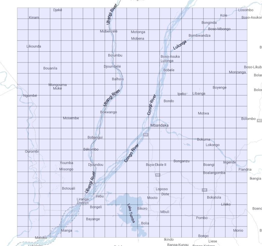
Let us discuss shortly the code proposed here: inside starting_point we define the coordinates of the starting point around which we are building up the grid and the number of decimal digits we are willing to keep after the truncation (this will clearly determine the size of each polygon). Then we are generating two arrays of integers spanning the interval [-10,10] in order to change iteratively the last decimal digit left after the truncation of both coordinates. This will give us the coordinates of the bottom-left corners of our polygons, from which it is straightforward to get the other three. The geography function st_makeline() and st_makepolygon() let us create eventually the geography containing the polygons. We finally get a 21x21 grid that looks as follows (Figure 1):
It looks nice!
Let us change the starting point:
with starting_point as(
select
  59 sp_lat,
  18 sp_long,
  1 digits
)
thus we get (Figure 2):
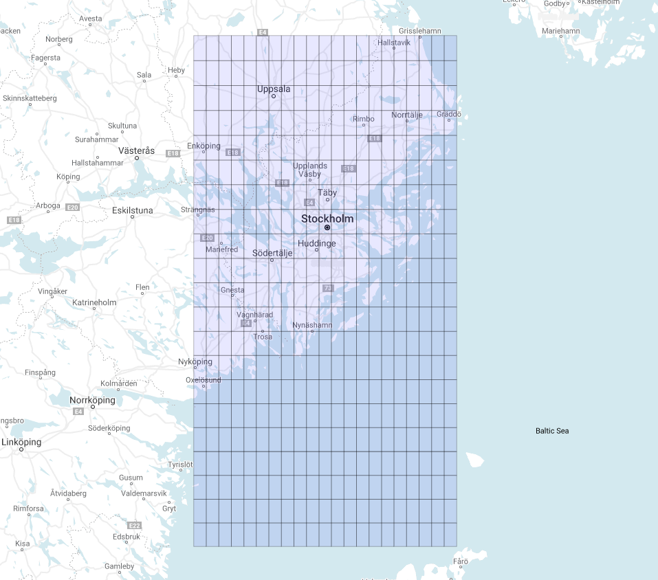
This grid looks a bit different from the last one. Why?
Remember that longitude and latitude are angular coordinates, and while moving 1° along a meridian (constant longitude) near the poles results in the exact same displacement as measured near the equator, the same does not apply for movements along parallels (constant latitude): as we approach the poles a change of 1° in longitude is progressively smaller and exactly 0 at the poles. We can easily convince ourselves of such a feature measuring the distance between any two vertices of the polygons as we vary the starting point:
st_length(st_makeline(st_geogpoint(pol_long,pol_lat),st_geogpoint(pol_long,pol_lat + pow(10,-digits)))) length_constant_longitude,
st_length(st_makeline(st_geogpoint(pol_long,pol_lat) ,st_geogpoint(pol_long + pow(10,-digits),pol_lat))) length_constant_latitude
You should note that the ratio between these two lengths is approximately equal to 1/cos(pol_lat), and that is why near the equator the polygons look like squares! Furthermore, taking this effect into account, we should expect the two grids to have the same height but different widths, i.e. a shorter base in the last grid shown. Surprisingly if we directly compare the two shapes on the map they look exactly the opposite! (Figure 3)
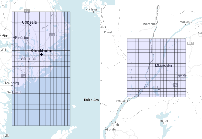
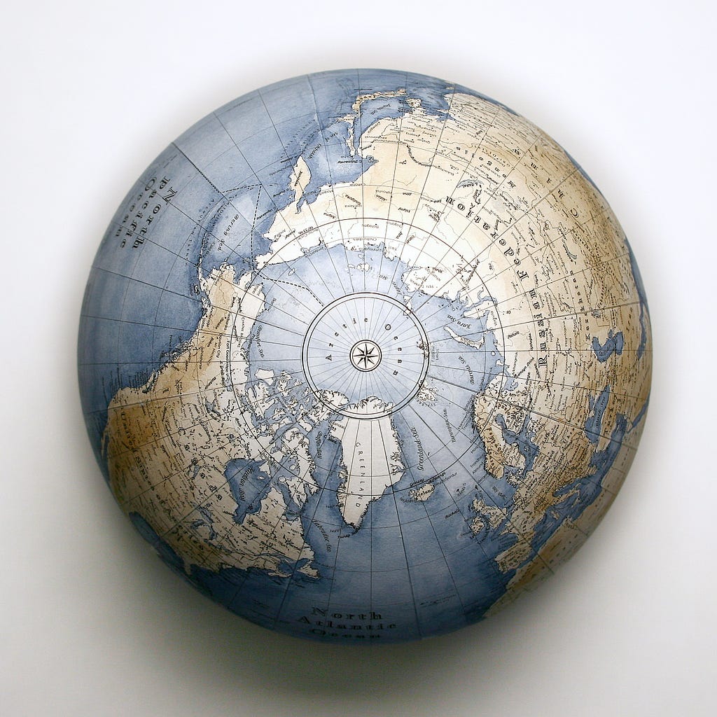
They have the same width but different heights. This is solely caused by the inevitable distortions of the projection used to map the curved surface of the Earth on a plane. This is why Greenland looks almost as big as Africa!
Creation of square bins
The binning technique just proposed is perfectly fine as any geographical point falls in one and only one polygon (which we will call tile from now on) of this grid (once extended to the whole surface), but it lacks the satisfying visual regularity of a grid made up of perfectly lined up squares (at least far from the equator!). A machine-learning algorithm may not care and, in that case, there are probably better solutions in which lengths or areas are kept constant throughout the grid, but if we are more interested in a tidy visual output then this solution fits better. Following the structure of the previous example we have:
with starting_point as( -- step 1
select
  0 sp_lat,
  18 sp_long,
  12 zoom
)
select
 zoom,
 tile_x,
 tile_y,
 st_makepolygon(st_makeline([
  st_geogpoint(ne_long,ne_lat),
  st_geogpoint(se_long,se_lat),
  st_geogpoint(sw_long,sw_lat),
  st_geogpoint(nw_long,nw_lat)])) polygon,
from( --step 3
 select
  zoom,
  tile_x,
  tile_y,
  180/acos(-1)*(2*acos(-1)*tile_x/pow(2,zoom)-acos(-1)) nw_long,
  360/acos(-1)*(atan(exp(acos(-1)-2*acos(-1)/pow(2,zoom)*tile_y))-acos(-1)/4) nw_lat,
  180/acos(-1)*(2*acos(-1)*(tile_x+1)/pow(2,zoom)-acos(-1)) ne_long,
  360/acos(-1)*(atan(exp(acos(-1)-2*acos(-1)/pow(2,zoom)*tile_y))-acos(-1)/4) ne_lat,
  180/acos(-1)*(2*acos(-1)*(tile_x+1)/pow(2,zoom)-acos(-1)) se_long,
  360/acos(-1)*(atan(exp(acos(-1)-2*acos(-1)/pow(2,zoom)*(tile_y+1)))-acos(-1)/4) se_lat,
  180/acos(-1)*(2*acos(-1)*(tile_x)/pow(2,zoom)-acos(-1)) sw_long,
  360/acos(-1)*(atan(exp(acos(-1)-2*acos(-1)/pow(2,zoom)*(tile_y+1)))-acos(-1)/4) sw_lat
 from( --step 2
  select
   zoom,
   trunc((sp_long*acos(-1)/180+acos(-1))/(2*acos(-1))*pow(2,zoom)) + x tile_x,
   trunc(pow(2,zoom)/(2*acos(-1))*(acos(-1)-safe.ln(tan(acos(-1)/4 + (sp_lat/180*acos(-1))/2)))) + y tile_y,
  from
   starting_point,
   unnest(generate_array(-10,10,1)) x,
   unnest(generate_array(-10,10,1)) y
     )
    )
This looks a bit more complex and lengthy, let us discuss each step:
- As in the previous example, we start both by defining the starting point around which we generate each tile of the grid and by choosing their desired size through the zoom parameter. What matters is that the lowest level of zoom is 0 (i.e. there is just one tile covering the whole map) and every time we go up a level the number of tiles quadruplicates. Here we arbitrarily choose a level of 12.
- We determine the “tile coordinates” of each square in the grid from the two arrays of integers. These coordinates and the zoom level will form together an unambiguous identifier for each tile. Note that we use acos(-1) to get the value of π.
- Next, we apply the inverse functions just used to get the coordinates of the four vertices of each square.
- Finally, we generate the tile as a geography data type using the usual geography functions. Note that these two last steps are necessary only if we want to visualize the grid on the map.
Thus we get this nice grid (Figure 4):
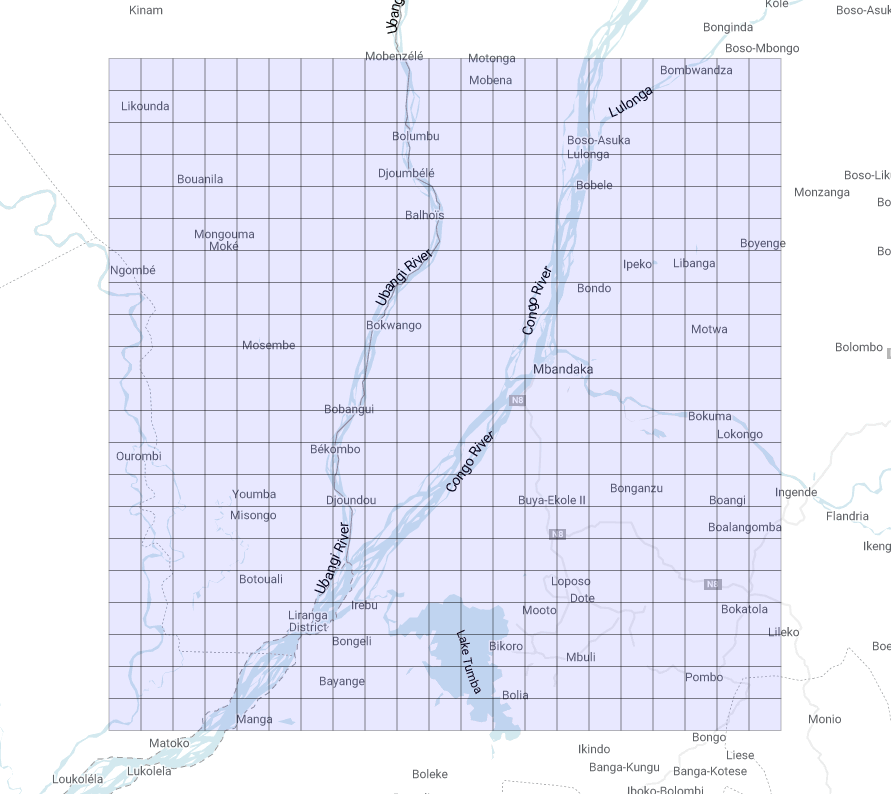
What if we change the starting point? Let us have a look (Figure 5):
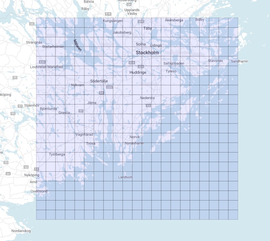
It is clear that we now have two identical grids made up of regular squares of the same apparent size, no matter where they are on the map. We want to stress once more that they only appear to be equal, when in fact they are not. The evaluation of their area reveals this feature: the average area of the tiles near the equator is about 95.5 km², while the average area of the tiles closer to the North Pole is about 25.3 km²!
We are finally ready to use this technique to create a lot of cool visualizations on both Geo Viz and Data Studio!
Enjoy! 😃
Spatial Binning with Google BigQuery was originally published in Towards Data Science on Medium, where people are continuing the conversation by highlighting and responding to this story.
from Towards Data Science - Medium https://ift.tt/3nZVK4z
via RiYo Analytics


No comments