https://ift.tt/30Z11lF SEAL Link Prediction, Explained Deep dive into the SEAL algorithm on toy data Graph Neural Networks (GNNs) have be...
SEAL Link Prediction, Explained
Deep dive into the SEAL algorithm on toy data
Graph Neural Networks (GNNs) have become very popular in recent years. You can do many things with them, like node label prediction, graph prediction, nodes embedding, link prediction and so on. This article aims to explain how SEAL (Subgraphs, Embeddings and Attributes for Link prediction) works by analyzing the implementation example code of one of the authors of the original paper, which can be found here : github.com/rusty1s/pytorch_geometric/blob/master/examples/seal_link_pred.py
Introduction
Link prediction is a really hot topic of research in the graph field. For example, given a social network below with different nodes connected to each other, we would like to predict whether nodes which are currently not connected will connect in the future. With graphs neural networks, we can use not only the information about the network structure, i.e. connections 2 given nodes have in common, but also the features of each node like hobbies they have, school they attended and so on.

Simple Graph
First, we will create some toy data to play with:
- edge_index : defines the edges between the nodes.
- x : nodes’ features (15 unique nodes in the toy data). Each node is going to have own features defined by the user (e.g. age, gender, bag of words and so on) concatenated to features defining the structural role of the node in each subgraph (it will become more clear in the next section).
- train, test, validation masks : Boolean mask arrays.
Enclosed subgraphs and nodes labelling
For each link in edge_index we need to extract the enclosed subgraph defined by the number of hops, source and target nodes, and label each node in each subgraph according to Double-Radius Node Labelling (DRNL) algorithm. This implies assigning a label to each node with the following formula :
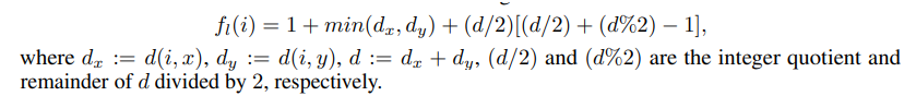
which depends on the distance (number of hops) between the node (i) and the source (x) and target (y) nodes.
This labelling method captures the structural roles of the nodes with respect to the source and target nodes, providing the model with more information to predict the link existence correctly.
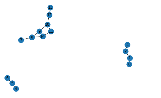
In the example above we illustrate the labelling for nodes 7 and 12 setting the number of hops to 2. Plugging into k_hop_subgraph function the two nodes and the edge_index of the entire graph we get as output the new sub_nodes (as we can see it includes all the sub nodes within 2 hops from source and target nodes), sub_edge_index (edge_index for the subgraph) and the z score for each node in the subgraph.
Z score is equal to 1 for the source and the target nodes. Nodes 11 and 14 have the same z score which is equal to 7:
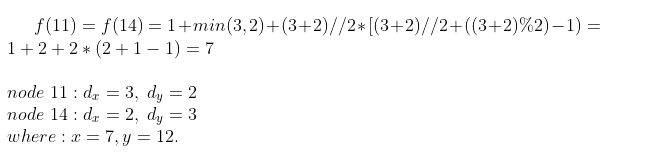
Because they have the same distance from the source and target nodes they have the same z score.
Now we need to split our data into train, test and validation, create negative examples and plug them all into a Dataloader [1]. The first part is straightforward — we remove some of the edges from the graph and use them for testing/validation. One thing we need to be careful about is not to split connected components into multiple ones. This check seems to be missing in the current implementation of the train_test_split_edges function. We also add the “undirected” parameter in order to remove the transformation to undirected and avoid duplicated subgraphs (subgraphs for [src=1, dst=2] is the same to [src=2, dst=1]). This allows to reduce the amount of ram required for the datasets. But we still want the undirected link between nodes to pass messages in both directions — we will come back to this later. To create negative examples, we pick randomly some edges which do not exist in the graph. In the current implementation, the strategy adapted is trivial and does not take into account information like distance between the nodes, nodes’ degree, nodes’ correlation and so on. Negative examples are very important in the optimization process to train a robust model, thus this should not be underestimated [2].
DGCNN model
In this part we will try to understand what DGCNN model is doing. We will go through one message passing analysing in details what is going on at every step. For simplicity we will assume:
- batch_size = 1
- normalization and bias = False (in GCNConv layer)
- number of GCNConv layers = 1
In the first place we calculate the parameter k, which is analogous to NLP maximum length of a sentence where we either truncate the sequence if the sequence length bigger than k or pad otherwise. Similarly here, each enclosed subgraph will have different number of nodes thus we will need to either truncate or pad. After that we do some adjustments to the elements in the dataloaders and apply the GCNConv layers:
1. As we removed from train_test_split_edges function the transformation to undirected subgraph to save space, we need to reintroduce it at this stage (line 90 in DGCNN.py file). In this way we do message passing in both directions. During the aggregation we also want to include the own features of the nodes, thus we add a self loop (line 91 in DGCNN.py file).
2. Transform original features with a weight matrix.
3. Compute new nodes’ features by aggregating the neighbours' features of each node (here the aggregating function is a simple sum).
4. Concatenate the convolutional layers.
5. Apply global sort pooling operation :
convolution operations which became very popular for features extraction from images have one major difference from the convolution operation to extract features from graphs : order of the nodes. Image pixels can be seen as nodes of a graph but they are naturally ordered, something that we lack in the graphs structure. From here comes the need for a consistent ordering of the nodes among subgraphs . Authors of the paper demonstrate that graph convolution operation approximates Weisfeiler-Lehman nodes coloring (an algorithm to compare different graphs by their colors/node labels patterns) and thus we can use the last layer of features from convolution operation to consistently sort the nodes, according to their structural roles in the subgraphs.
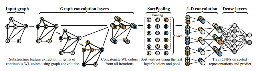
After the sorting, we standardize the number of nodes for each subgraph , truncating the sorted sequence of nodes if k is less than number of nodes and pad otherwise [3].
6. After we have done the sorting according to WL colors we have a structured data as in images, so we can apply 1D convolution, max pooling and linear layers to eventually predict the existence of a link between 2 nodes.
Conclusion
In this article we described all the steps of the SEAL algorithm — from nodes labelling to message passing with graph convolutional operations on some toy data. We have also seen the analogy between image and graph structured data that enable us to apply the convolutional operations on graphs. As the next step, we will be fitting the algorithm to some real data assessing how different strategies of picking negative examples affect the performance of the algorithm.
References
[1] stanford.edu/~shervine/blog/pytorch-how-to-generate-data-parallel
[2] arxiv.org/pdf/2005.09863.pdf
[3] muhanzhang.github.io/papers/AAAI_2018_DGCNN.pdf
SEAL link prediction explained was originally published in Towards Data Science on Medium, where people are continuing the conversation by highlighting and responding to this story.
from Towards Data Science - Medium https://ift.tt/3ldQR7s
via RiYo Analytics


ليست هناك تعليقات