https://ift.tt/3qUMfHd …and why do R and Stata get all the fun? What do you do if your data takes some really weird shapes? Like, really w...
…and why do R and Stata get all the fun?
What do you do if your data takes some really weird shapes? Like, really weird? Other than say “#@&% it” and decide to use a decision tree? Once you learn nonparametric models, it is very easy to think that parametric models are too clunky to seriously consider for more complex modeling projects. As you may or may not know, nonparametric models like decision trees, K-nearest neighbors, and others offer a significant advantage in that they make no assumptions about an underlying distribution or equation like a parametric model does. It’s in the name — parametric models attempt to find the parameters or some equation or line that best describes the data, and this is not an undertaking that one makes lightly! Indeed, it is very rare that data in the wild takes nice, comfortable linear forms:

More frequently, you get nightmare data like this:

You might think that parameter estimation is overly limiting and doomed to produce inadequate results. So how do you deal with this? As I mentioned above, you could eschew parametric modeling altogether, but that comes with its own set of problems. Sometimes, you really just have to suck it up and use a parametric model. And since you have a creatively-shaped set of data points, you need to get creative with your methods to model it. This is where Multivariate Fractional Polynomials (MFP) come in.
I came across this technique (and function in R and Stata) while researching my previous blog post, and ended up reading so much about it that I decided it was best to save it for its own post. I’m actually quite surprised that there’s not more information about it out there on the net — it seems that most discussions about it or papers using it are limited to certain statistics spaces and the medical science community. I would think that due to its huge potential it would be used in other places, or at least available as a Scikit-learn-style utility. But there's not! There’s not even a discussion of its use in Python out there, which I find greatly puzzling.
So really, the point of all this is to put this on your radar as a powerful tool that exists. The MFP algorithm combines complex feature engineering and selection all in one go, done in a neat, programmatic, and statistically sound fashion. Who could ask for more? In this blog post, I’ll take you through the various papers I stumbled upon and walk you through the general idea, rhapsodize on its power, and point to where you might acquire it for use.
But before I get into the details of MFP, a brief primer on parametric modeling…
Parametric Modeling
The whole idea behind this is that you need to get some kind of line to fit a bunch of data points. This is maybe best exemplified in Linear Regression, which is described by an equation like so:

Graphically in 2D, you could model the nice data from the first figure above like this:

For many variables, this line would exist in many more dimensions than we could imagine with our crude 3D brains, but it works in the same way.
One dependent variable is the output of potentially many independent input variables. Note that from now on, I’ll be speaking for solely continuous variables: those which can take on any numerical value within a range. The barebones baseline assumption you start with is that the independents (X, above) are first-degree — which is to say, to the first power. But you need not limit yourself. There is room for experimentation with the independent variables in order to make the relationship more linear, and this is the realm of feature engineering. You can create interaction terms, polynomial features, log transformations, really any kind of transformation of the raw data you started with. The sterling Scikit-learn, in its infinite utility, has some functions to assist in that: PolynomialFeatures, most notably. For the uninitiated, it enables you to, in one line of code, create a bunch of new features by multiplying all the originals together or with themselves. Like, if you had features A, B, C, you could make degree 2 polynomial features of A*B, A*C, A², B*C, B², C².
However, other than the aforementioned utility, it’s not easy to programmatically create nonlinear features, and it usually requires some degree of domain expertise to know what to look out for. But that also takes some guesswork, and it’s extremely unlikely you’ll be able to think of extremely complex and descriptive engineered features no matter how much you know the domain. And from the PolynomialFeatures side, just making a boatload of features is going to lead to other issues since only a small fraction are actually important. This sort of shotgun method demands some robust feature selection in order to remove all of the unnecessary complexity you just added in and leave the truly important complex terms.
What if we could create some extremely complex terms and remove unnecessary complexity?
Multivariate Fractional Polynomials (MFP)
As far as I can tell, this technique was first published in 1994, coming to us from the Journal of the Royal Statistical Society, by Patrick Royston and Douglas G. Altman. In the paper’s summary, they describe some of the same weaknesses I described above, as well as others, giving a complete portrait of the failings of traditional curvature solutions. They then propose a solution as an “extended family of curves…whose power terms are restricted to a small predefined set of integer and non-integer values. Powers are selected so that conventional polynomials are a subset of the family.” This list contains the most important features you could engineer for a variable. They then go on to say that this is more or less a formalization of something that had been appearing in literature for a while up to that point and assert MPF’s flexibility and ease of use. Later in the paper, they suggest an algorithm for iteratively selecting the powers in this family for each dependent variable. This is where the critical feature selection component I mentioned above comes in, since it includes backward elimination as part of the process. The paper closes with several examples from medicine — perhaps an interesting premonition of the technique remaining squarely in that field even today. I won’t delve into the various examples from this paper (and others that follow below), but please do look at how this technique works with real-world data. It’s quite interesting. Also if you’re itching for more examples, a simple search of “Multivariate Fractional Polynomials” yields a good number of them from medical data spaces.
“Family of Curves”: Feature Engineering Made Easier
We’ll first dig into their basic setup for what that “family of curves” is, and then dive into the iterative algorithm that they propose. This paper from Duong et al. (2014) offers a much better summary than anything I could’ve come up with. There is a predefined set S = {-2, -1, -0.5, 0, 0.5, 1, 2, 3} which contains all of the possible powers for your independent variables (0 is defined as ln(X)). Your variables can take the form X^p (degree 1) or X^p1 + X^p2 (degree 2) for different values of powers (p, p1, and p2), taken from that set S. Technically, this could be expanded to more than two degrees, but Royston and Altman suggested that that’s unnecessary. These two degrees of Fractional Polynomial (FP) are constructed thusly:
FP degree 1 with one power p:
y = β0 +β1X^p
(when p=0): y= β0 +β1ln(X)
FP degree 2 with one pair of powers (p1, p2):
y = β0 + β1X^p1 + β2X^p2 (same rules with p=0 applies)
(when p1=p2): y = β0 + β1X^p1 + β2X^p2*ln(X)
From this construction, FP1 has 8 models with 8 different power values, and FP2 has 36 different models — 28 combinations of those 8 values and 8 repeated ones. Altogether, we get 44 possible models with which we can fit our data. Critically, it’s important to keep in mind that these are just jumping-off points, and the values of the β-coefficients will also change the shape of these lines quite severely (see below).
So what? It’s probably hard to see the value in this just based on equations; I hear you. A visual demonstration might best explain why these 44 models are so darn effective. While you look at the following graphs, ponder a moment on how complex the line traces are, and how much of a headache it would be to try to think this up alone, just by staring at scatterplots.
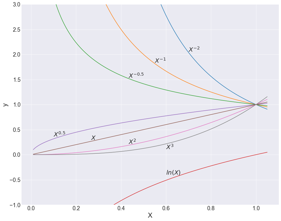
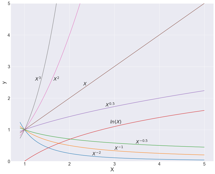
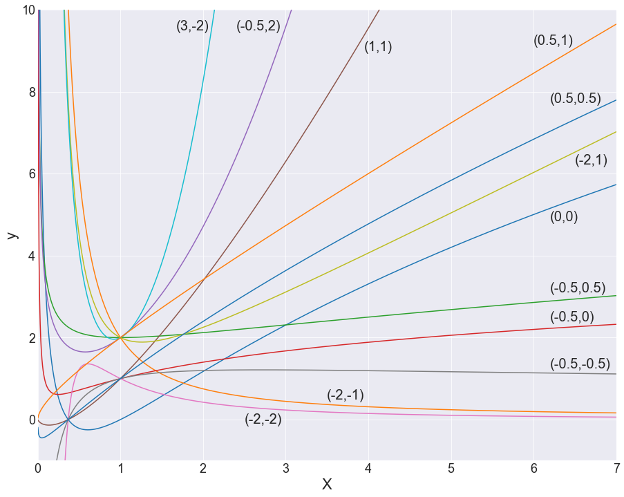

With any hope, you’d come to the same conclusion I did, which is that coming up with this unassisted is pretty much impossible! And that’s really where the power in feature engineering comes from — this method provides a set of the most descriptive powers for our independent variables, along with a structure with which to put them together. And this would be enough, but the method also comes with a feature selection component.
Built-in Feature Selection
Again, I’ll use someone else’s clear explanation to cover this, coming from both Duong and Zhang, et al (2016). Zhang outlines the general procedure for how to select the proper degree and correct powers for your independent variables. It first points out that there are two components to the process:
- Backward elimination of statistically insignificant variables
- Iterative examination of a variable’s FP degree
Accordingly with the above two pieces, you need two significant levels: α1, for exclusion/inclusion of a variable, and α2, to determine the significance of a fractional transformation. Note that a1 and a2 can be (and is often) the same value, but it is something you can play around with.
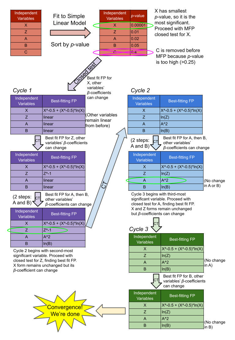
So, with your α values and list of continuous variables, you begin by building a multivariable linear model with all variables together. Alternatively, you can do a univariable analysis of each variable with the target, and only include those with p<0.25 or 0.2, to help pare down truly unimportant variables. You then organize all the variables in order of increasing p-value from that first model.
Next, you take the top, lowest p-value variable and begin the closed test, which tracks how changing the variable’s form affects the full model’s fit (aka it’s not a univariable model). This proceeds as follows (details on statistical tests from Duong):
- Find the best-fitting second-degree fractional polynomial (FP2) for that variable, based on deviation (aka model error). Compare that with the null model (where the variable is not present) using a chi-squared difference test with 4 degrees of freedom. If the test is not significant (according to α1), drop the variable and conclude there is no effect of the variable on the target. Otherwise, continue.
- Compare the FP2 model from step 1 with the linear model (variable power = 1) to determine non-linearity, using a chi-squared difference test with 3 degrees of freedom. If the test is not significant (according to α2), the variable is linear and the closed test ends. Otherwise, continue.
- Find the best-fitting first-degree fractional polynomial (FP1) for the variable, similar to step 1. Compare that with the FP2 model using a chi-squared difference test with 2 degrees of freedom. If the test is not significant (according to α2), the model does not benefit from additional complexity, and the correct model is FP1.
(For more information on why we use Chi-squared difference tests to evaluate these models, look here)

Now, once you’ve performed the above closed test for the lowest p-value variable, you then go through and do the same assessment for the next highest p-value variable from that ordered list you generated earlier in the original big linear model. The FP form of the previous X is retained but the β-coefficients can change in response. This continues sequentially for every other variable, and this marks cycle one. Cycle two is the same procedure, just starting with the second-lowest p-value variable, and keeping the previous low p-value variable’s FP form. This cyclic process continues iteratively until two cycles converge and no changes are made.
More Complexity, for the Stubbornly Complex
If your data is somehow particularly bananas, and may God have mercy, there are other things you might consider doing with your fancy new FPs in tow. They’re probably complex enough, but you could consider multiplying FPs together a la PolynomialFeatures. Similarly, you might decide to eschew the MFP decision algorithm (directly above) altogether and simply make polynomial features out of variables with powers in the FP set S (= {-2, -1, -0.5, 0, 0.5, 1, 2, 3}, with 0 as ln(X)). Given the inclusion of negative powers, ln, and square root, this would probably still offer you a fair deal of additional modeling power compared to base PolynomialFeatures. Of course, either of the above decisions will likely require additional feature selection.
Drawbacks, Since Not Everything Can Be Perfect
As far as I can tell, the main drawback to MFP lies in how computationally expensive it is. But I suppose this isn’t terribly surprising given how many steps you need to go through to find the ideal FP form for each feature — in a typical scenario, the selection algorithm would require 44 models to be calculated for comparison, for each feature, which could take quite a bit of time. But placed in context, models that can capture similar levels of complexity (a grid-searched Random Forest or a neural network, for example) would probably not fare that much better. Furthermore, with some of these other models, the run time will be reduced but you’ll sacrifice interpretability down the line. MFP seems to strike a good balance.
In addition, MFP seems to ignore interaction terms, which may weaken its overall strength as a tool. If two variables have a synergistic effect, MFP will ignore them as the algorithm is performed. An easy way to get around this would be to feed in interaction terms at the start, but adding features will increase the runtime of an already expensive process, as I mentioned just a moment ago. Alternatively, as I laid out in the preceding section, you might just forgo the built-in selection algorithm altogether and try out a PolynomialFeatures sort of workflow, simply using powers in the FP set S. Definitely something to play around with to see what works best.
Cut to the Chase — Where’s the Python Package?
Thank you for reading this far, I know that was a fair bit of detail. Unfortunately, I don’t have any good news for you on the other side. It would seem, based on a fair bit of searching, that there is no easy way to incorporate this into a Python-based data project. I apologize for all the build up with no payoff — in many ways, this post is an expression of my own frustration. As I mentioned in the introduction, there is not much discussion (if any, really) about this very powerful method outside of medical statistics contexts, even though its broad utility is plainly obvious. It does exist as a function in R and Stata, but unless I’m missing someone’s obscure GitHub repo, it doesn’t exist in any Python package, which I find frankly shocking. The closest thing in Python to modeling this level of curve detail is Scikit-learn’s spline functionality, which seems to do a bang-up job — but that can be difficult to work with in its own right, and there are clear advantages to the MFP approach.
It really sucks how this technique is squirreled away from the rest of the statistical world, and with any luck, this post might inspire some change. Perhaps I’ll be the change and write a Scikit-learn-style utility to perform MFP and supercharge my parametric models, and when I do that I’ll make sure to link the GitHub repo below. But in the meantime, if you, dear reader, are in dire need of this functionality now, hopefully you’d be able to use the resources I’ve laid out in this post as a jumping-off point to build your own function in the meantime.
References:
Royston, P., & Altman, D. G. (1994). Regression Using Fractional Polynomials of Continuous Covariates: Parsimonious Parametric Modelling. Journal of the Royal Statistical Society. Series C (Applied Statistics), 43(3), 429–467. https://doi.org/10.2307/2986270
Duong, H., & Volding, D. (2014). Modelling continuous risk variables: Introduction to fractional polynomial regression. Vietnam Journal of Science, 1(2), 1–5.
Zhang Z. (2016). Multivariable fractional polynomial method for regression model. Annals of translational medicine, 4(9), 174. https://doi.org/10.21037/atm.2016.05.01
Multivariate Fractional Polynomials: Why Isn’t This Used More? was originally published in Towards Data Science on Medium, where people are continuing the conversation by highlighting and responding to this story.
from Towards Data Science - Medium https://ift.tt/3kAsBfq
via RiYo Analytics


No comments