https://ift.tt/3EYqw4L The theory behind LES and its use in computational fluid dynamics. Have you ever wanted to simulate how physical ob...
The theory behind LES and its use in computational fluid dynamics.
Have you ever wanted to simulate how physical objects interact with air and water? Here’s how.

Large Eddy Simulations (LES) is a cutting-edge technique that is used to simulate how hardware interacts with fluids. It strikes a balance between computational efficiency and granularity, which has led to tremendous popularity in the aerospace and automobile industry. However, they are not a silver bullet, yet.
In this post, we will discuss the basics of LES. If you want a code tutorial, leave a comment.
Without further ado, let’s dive in.
Technical TLDR
Large Eddy Simulations (LES) are computationally “efficient” simulations that solve the Navier-Stokes equations. The main computational benefit comes from filtering, which chunks our data into computationally feasible blocks. For information in each block, we directly solve the equations and for smaller Sub-Grid Scale (SGS) data, we can develop approximate models.
But what’s actually going on?
If you’re not a physicist with a math background, that may have been a lot so let’s slow down a bit.
1 — Navier-Stokes Equations
We’re going to start with a tangible example: we’re looking to design the shape of a ship propellor that maximizes forward thrust.
In developing this propellor, there would be two main paths forward. The first would be to leverage our knowledge about ship propellor physics and come up with theoretical designs. Unfortunately, not many of us are experts in fluid dynamics, so that option may be problematic.
Instead, let’s discuss a second option: Large Eddy Simulations (LES).
LES can combine physics and computational simulation to estimate properties about water flow which can then be translated into estimates of thrust. The core of LES relies on the two Navier-Stokes equations which govern all fluid dynamics.
Let’s discuss each equation in turn.
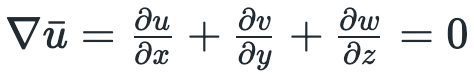
1.1 — Conservation of Mass
The first equation is pretty intuitive. It states that no matter how much we move our fluid, the mass of the fluid will remain the same.
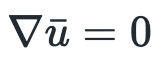
In figure 1, u_bar (the u with a bar over it) corresponds to the velocity of our fluid. Velocity includes both a speed and a direction and in our case, were interested in all 3 dimensions of thrust, so let’s break down u_bar into an x, y, and z component.
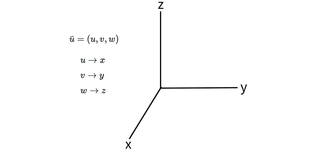
As shown in figure 2, we can decompose u_bar to it’s u, v, and w components, which correspond to the x, y, and z directions of our velocity. The magnitude of each of these three components corresponds to the speed in that direction.
Now that we understand the velocity term, let’s look at the nabla (∇). ∇ indicates that we are looking at the gradient in our velocity. If you’re familiar with stochastic gradient descent, this gradient is the same concept — it’s just the partial derivatives of velocity with respect to x, y, and z.
1.2 — Conservation of Momentum
The second of the two equations is also very intuitive. It simply states that all momentum in a system will be preserved through time. It also happens to be Newton’s second law.
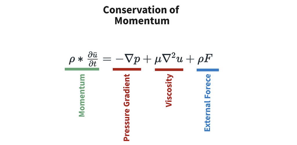
In figure 4, the value on the left side of the equal sign (green) is momentum. It’s just our fluid density ρ (rho) multiplied by the rate of change of u_bar over time. It’s good to note that this term is just a different representation of mass x acceleration.
The two values in red are internal forces — they correspond to interactions inherent to fluid particles. The first term, the pressure gradient, is the pressure that disperses particles from high density to low density areas. For an example, think about how smells disperse and dissipate in a room. The second term, viscosity, is the “thickness” of a substance and corresponds to friction between particles in the fluid.
Finally, we have our only external force, shown in blue. This is often just replaced with the gravitational constant.
Fun fact of the day, if you can prove that solutions to these equations exist and are smooth, you win a million dollars.
2 — The Problem of Turbulence
When looking to solve the above equations, there is one main challenge: turbulence.

Turbulence, artistically shown above, is “motion characterized by chaotic changes in pressure and flow velocity.” Each particle in our fluid could theoretically contribute to turbulence so unless we have extremely powerful computers (like atomic computers), we won’t be able to solve the above equations.
So, to reduce computational complexity, we filter out certain portions of our data. There are three primary “versions” of the Navier-Stokes equations with differing levels of granularity and thereby computational complexity. They are…
- Direct Numerical Simulation (DNS): no filter — only suitable for small scale theoretical simulations.
- Large Eddy Simulations (LES): filter out and model small scale “eddies” — very precise method that’s still computationally tractable.
- Reynolds-Averaged Navier-Stokes (RANS): filter values below a threshold by averaging them — a less precise method that’s more computationally efficient than LES.
Historically, RANS has been the state of the art method but with increased computational power, LES has seen a surge in popularity for applications where precision is necessary. One example would be internal combustion engine design.
3 — Large Eddy Simulations
Now that we understand why computational fluid dynamics simulations can be very expensive, let’s see what we can do in practice to reduce its complexity.
3.1 — Low-Pass Filtering
A simple explicit filtering method used in LES is called low-pass filtering. As you’d expect, we reduce or remove high frequency signals and let low-frequency signals pass by unchanged. “High” and “low” are determined by a threshold Δ (delta).
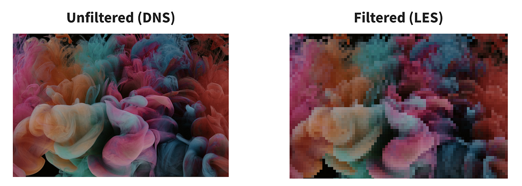
A simplified analogy for this process is pixelating images, as shown in figure 5. We achieve this “pixilation” by using a convolution kernel. Similar to a convolutional layer in CNNs, we move over our data using a sliding “window” and perform a low-pass filtering operation at each location. Also note that we don’t just do this for 2D data — we also can apply this data to 3 dimensions as well as our temporal component.
From a visual perspective, filters applied to spacial components in our data are often represented by a mesh overlaid onto our data. Each grid cell in figure 6 corresponds to the output of a convolution kernel (or some other filtering method).

As hinted at above, there are tons of other filtering methods. Some explicitly determine the size of a signal that should be allowed to pass through whereas others leverage complex math to dynamically reduce the amount of small turbulent processes. There are also sub-grid scale (SGS) models that try to encapsulate relevant information about turbulence in a computationally efficient manner.
3.2 — Solving the Navier-Stokes Equations
Now that we have a computationally tractable dataset, we can apply calculus-based solvers and thereby perform simulations. The math and code can get super complex, so here are some resources if you’re curious to learn more:
- Stanford High Fidelity LES: research-oriented LES designed by the Aerospace Computing Laboratory
- dedaLES: most popular python library for LES
- ARXIV.org: a good (and free) way to stay on top of LES research
And there you have it — LES in all it’s glory!
Summary
To hammer home some concepts, let’s reiterate what we discussed above then connect our new knowledge to some cool applications.
Large Eddy Simulations (LES) are computationally intensive yet tractable simulations of fluid dynamics. Their claim to fame is that they use filters to remove small-scale turbulence, which causes of much of the computational complexity. From there, it leverages efficient and ideally parallelized solvers to determine solutions for the Navier-Stokes equations.
LES has become extremely popular in the hardware modeling space. Some applications include internal combustion engines, aerospace engineering, wind turbine design, and marine energy. By leveraging computers, we can theoretically test thousands of possible designs prior to building a physical prototype.
Thanks for reading! I’ll be writing 28 more posts that bring academic research to the DS industry. Check out my comment for links to the main source for this post and some useful resources.
Large Eddy Simulations was originally published in Towards Data Science on Medium, where people are continuing the conversation by highlighting and responding to this story.
from Towards Data Science - Medium https://ift.tt/3D12F3T
via RiYo Analytics


ليست هناك تعليقات