https://ift.tt/3Hwmh2q An overview of the InterpretML package, which offers new explainability tools along side existing ones. Photo by V...
An overview of the InterpretML package, which offers new explainability tools along side existing ones.

Interpretability can be crucial when implementing ML models. By interpreting models , customers can gain trust in the model and facilitate adoption. It may also be helpful in debugging your model, and in some situations, you will be required to provide explanations for predictions generated by the model. In my previous blog post, I discussed two methods: LIME and SHAP, that I used in one of our projects at Dell.
In this blog post, I’ll provide an overview of the InterpretML package, which holds a new developed interpretable model (Explainable Boosting Machine) that can explain your model in both a global and local context, alongside existing methods like LIME, SHAP, and more with great visualizations that can take your model’s explanations to the next level.
This blog will cover the following:
- InterpretML overview
- Explainable Boosting Machine (EBM)
- Examples
- Summary
- Further reading
1. InterpretML Overview
InterpretML is an open-source Python package that contains different interpretability algorithms which can be used by both practitioners and researchers. The package offers two types of interpretability methods: glassbox and blackbox. The glassbox methods include both interpretable models such as linear regression, logistic regression, decision trees that can be trained as a part of the package, as well as corresponding explainability tools. While the blackbox models only include model-agnostic explainability tools such as LIME, and Kernel SHAP that are compatible with models trained outside the package, the glassbox models provide both global and local explanations, while the blackbox models only support local explanations. Furthermore, InterpretML has a built-in visualization platform that allows users to compare different methods easily. Moreover, as InterpretML is scikit-learn compatible, the hyperparameters of the glassbox models can be tuned as other scikit-learn models. To emphasize the difference, using a glassbox model in your project, will allow you to both train and visualize explanations using InterpretML, while using a different model will only allow you to visualize explanations generated by a blackbox model, after training the model with another package.

Lastly, the package also includes a new interpretable model- Explainable Boosting Machine (EBM) that was developed by Microsoft Researchers and will be discussed in the next section.
2. Explainable Boosting Machine (EBM)
EBM is a glassbox model indented to have comparable accuracy to machine learning models such as Random Forest and Boosted Trees as well as interpretability capabilities. EBM is a Generalized Additive Model (GAM) which is very similar to linear models. In linear models, the relation between the observations Y and the dependent variables Xi is formulated as:
Y = β0 + β1X1 + β2X2 + β3X3 + … + βnXn
while in Generalized additive models, the relation is formalized as:
Y = β0 + f(X1) + f(X2) + f(X3) + … + f(Xn)
So now each contribution to the predictor is now some function f. EBM offers some improvements to traditional GAMs: each feature function is learned using modern machine learning technique such as bagging and boosting. Training is carried out in many iterations where each iteration consists of constructing a boosting procedure separately for each feature. As this is done with low learning rates, the order of the features does not matter. The high number of iterations aims to mitigate the effects of co-linearity in order to learn best what is the contribution of each feature to the model’s prediction. Furthermore, EBM can automatically detect and include pairwise interaction terms, this increases the accuracy of the model while preserving its explainability. Since EBM is an additive model, the contribution of each feature can be captured and visualized, and therefore enhance explainability.

As a further explanation, for each iteration of the model, small trees are constructed sequentially and each tree can only use a single feature, in a boosting manner the residual is updated and a new tree is constructed using a different feature. This is done for each feature in every iteration. Once training is completed, we can look at all the trees that were constructed by a certain feature, and build a graph based on their predictions that showing the contribution that each feature made to the predictions.
3. Examples
As an example, we will use the heart failure prediction data set from Kaggle. The data set contains 12 features that can be used to predict mortality (DEATH_EVENT- 0/1) by heart failure. Some of the features include: age, sex, whether the patient has anemia/diabetes/high blood pressure and more.
We will Examine the following models and corresponding explanations generated by InterpretML:
- EBM (glassbox)
2. Logistic Regression (glassbox)
3. LightGBM using Lime and SHAP (blackbox)
A notebook of the code, including the interactive visualizations can be found here.
Before getting into the examples, it is important to note that unlike the implementations of LIME and SHAP, for classification problems with EBM / logistic regression, the contributions of features are expressed as log odds and not probabilities. In fact, as done in logistic regression, to get the probability, the log odds is passed through a logit link function. Scores are displayed in an additive log odds space because it allows a fair comparison of the contributions from each feature. This is due to the non-linearity of the log odds and the probability. Look into this GitHub issue for more information.
Following that I will share some examples of what else you can do with InterpretML beyond explainability.
EBM
Let’s start by looking at the global explanation.
ebm_global = trained_ebm.explain_global()
show(ebm_global)
You can look at the overall importance of the features, and also look into each feature/interaction separately.

The overall importance of each feature is the average of the absolute predicted value of each feature in the training set. Essentially, each data point in the training data is scored using one feature at a time. The absolute values of the scores are averaged, this creates each bar in the summary plot.

As mentioned before, you can look into each feature individually and see how the value of the feature affects the score. You will also notice grey markup, these are the error bars. These are estimates of the model’s uncertainty within certain regions of the feature. The broader the bar, the greater the impact of small changes in the training data. Based on that, interpretation of these data points should be addressed with caution. You can access the the error bar sizes with the following code:
trained_ebm.term_standard_deviations_[4]
This will give us the standard deviations of the fourth feature in the data.
Now, let’s look into the local explanation. You can examine several observations together using the following code:
ebm_local = trained_ebm.explain_local(X_test[10:15], y_test[10:15])
show(ebm_local)
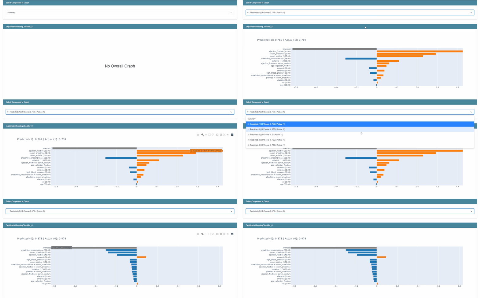
To generate the local predictions, the model uses the graph created for each feature as a lookup table together with the learned intercept.
Logistic Regression
Let’s start by looking at the global explanation:
lr_global = trained_lr.explain_global()
show(lr_global)
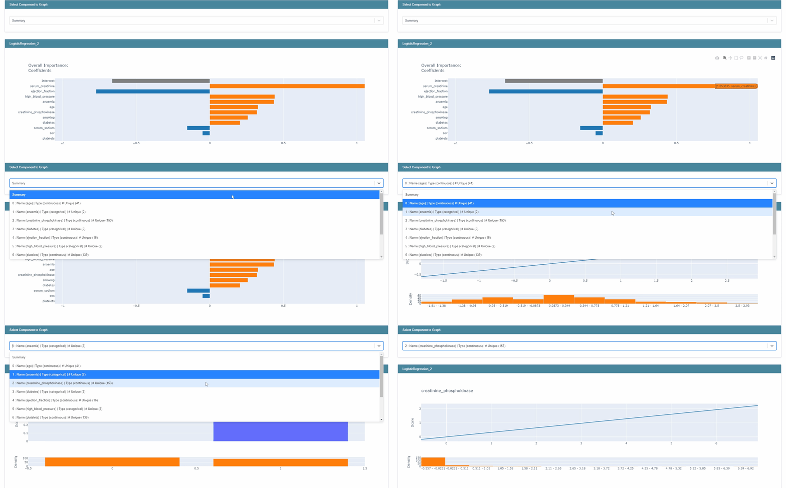
Here, as opposed to EBM the global explanation not only provides the magnitude but also the sign. As before, you can examine each feature separately as well.
Now, let’s examine the local explanations:

Now, you can compare the local explanations provided by the EBM model with the local explanations provided by the logistic regression model.
Based on your knowledge or with the help domain experts you can decided which one is a better fit.
LightGBM using LIME and SHAP
Depending on the data, you might want to use a model other than EBM or logistic regression. One example of such reason could be the presence of missing values in the data- while LightGBM is able to handle the presence of missing values, other models may requires filling the missing values prior to training.
As opposed to previous presented methods, using the InterpretML package, you cannot generate global explanations to a non-glassbox model. However, using SHAP directly will allow you to do that. Another important point to note is that using SHAP through InterpretML, only provides KernalSHAP which is model agnostic. Using SHAP directly offers additional explainers such as: TreeSHAP and DeepSHAP.
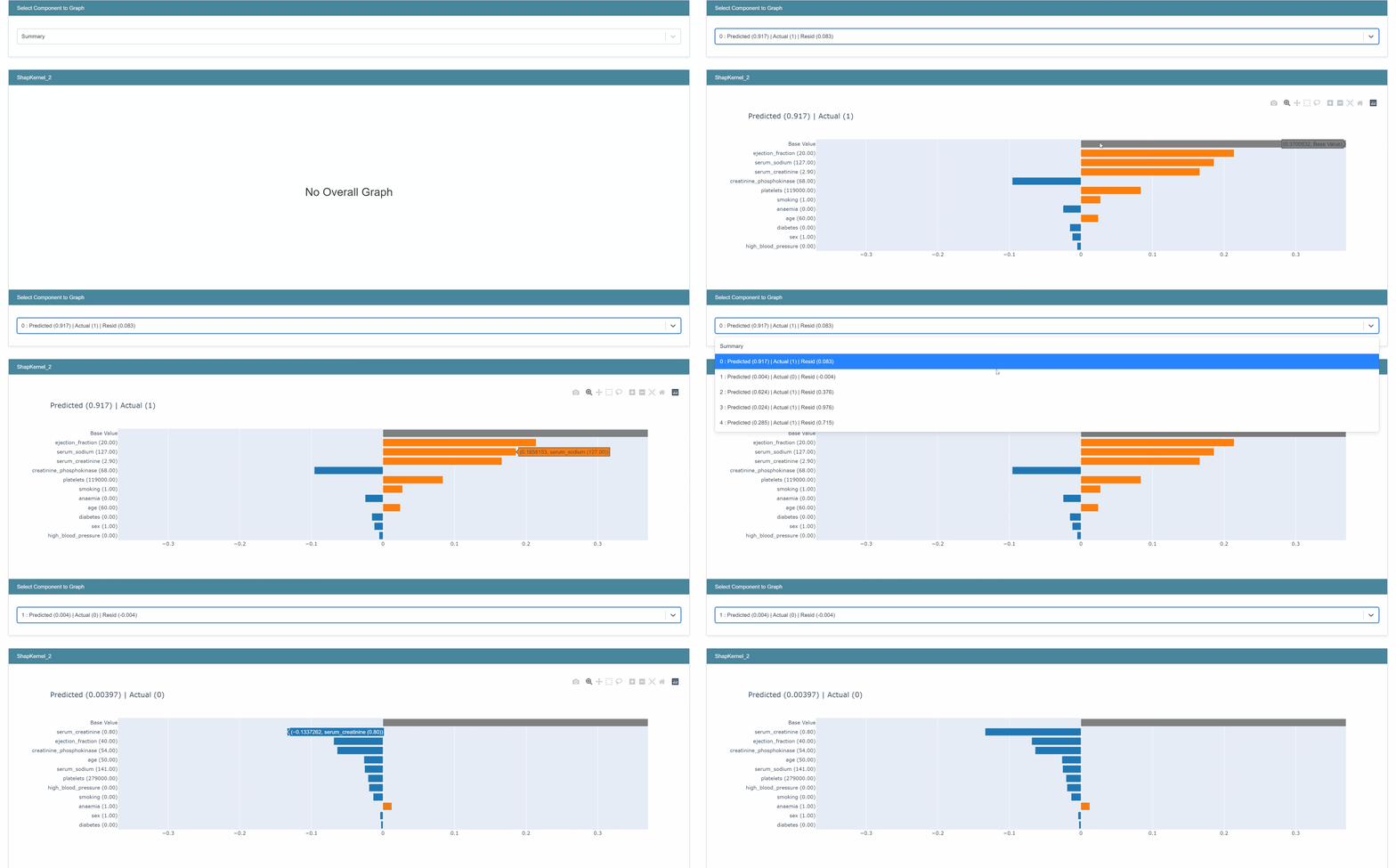
we will start by looking into SHAP:
from interpret.blackbox import ShapKernel
shap = ShapKernel(predict_fn=trained_LGBM.predict_proba, data=X_train)
shap_local = shap.explain_local(X_test[10:15], y_test[10:15])
show(shap_local)
Now, let’s look into LIME:
lime = LimeTabular(predict_fn=trained_LGBM.predict_proba, data=X_train)
lime_local = lime.explain_local(X_test[10:15], y_test[10:15])
show(lime_local)

As you can see, the local explanations for both the glassbox and blackbox models have the same format.
Notice that if you have categorical features in the data that were one-hot-encoded, results might not be entirely reliable. This is because LIME creates explanations by permuting data. If the features are one hot encoded, LIME cannot know which columns are a part of the same original feature, and as a result create a data point that is not consistent with the original data.
To know more about SHAP, LIME and how to deal with categorical data, check out my previous blog post.
InterpretML beyond explainability
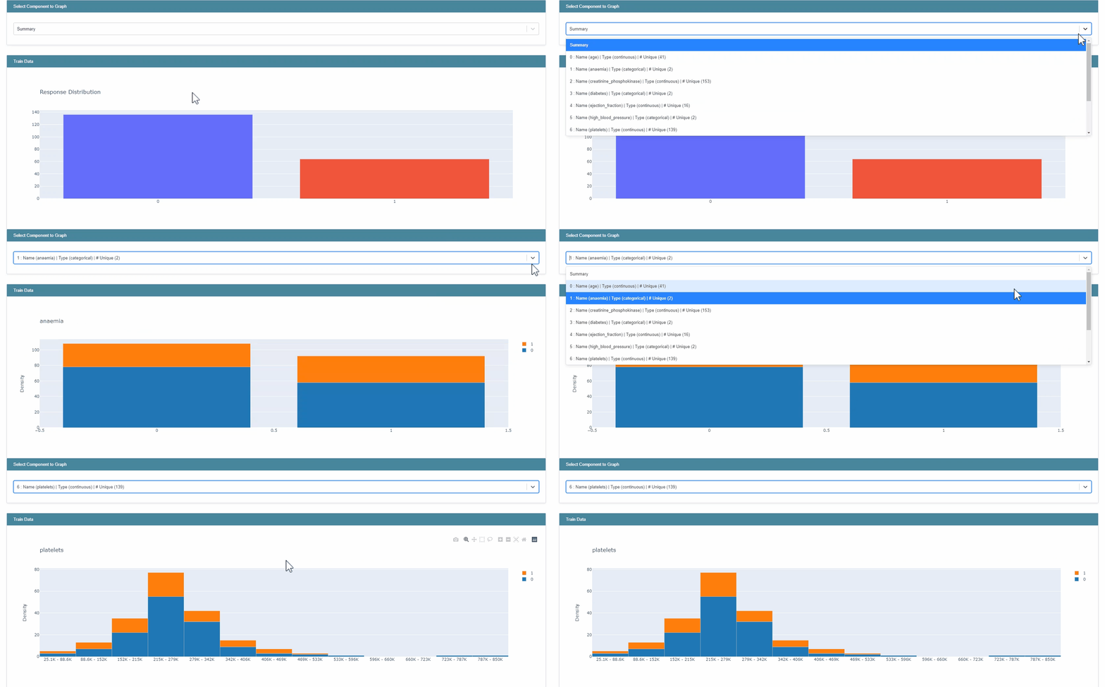
InterpretML can be used to perform EDA on the data, the package offers some basic EDA capabilities using plotly.
from interpret import show
from interpret.provider import InlineProvider
from interpret import set_visualize_provider
set_visualize_provider(InlineProvider())
from interpret.data import ClassHistogram
hist = ClassHistogram().explain_data(X_train, y_train, name="Train Data")
show(hist)
You can also perform hypermeter tuning of models in the package. Here as an example, I used RandomizedSearchCV with 3 fold cross validation.
from interpret.glassbox import ExplainableBoostingClassifier
from sklearn.model_selection import RandomizedSearchCV
param_test = {'learning_rate': [0.001,0.005,0.01,0.03],
              'interactions': [5,10,15],
              'max_interaction_bins': [10,15,20],
              'max_rounds': [5000,10000,15000,20000],
              'min_samples_leaf': [2,3,5],
              'max_leaves': [3,5,10]}
n_HP_points_to_test=10
LGBM_clf = LGBMClassifier(random_state=314, n_jobs=-1)
LGBM_gs = RandomizedSearchCV(
    estimator=LGBM_clf,
    param_distributions=param_test,
    n_iter=n_HP_points_to_test,
    scoring="roc_auc",
    cv=3,
    refit=True,
    random_state=314,
    verbose=False,
)
LGBM_gs.fit(X_train, y_train)
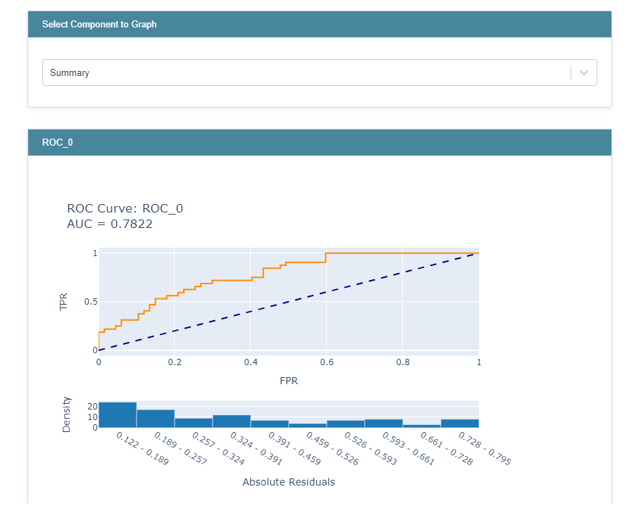
You can use the following code to further compare the results by plotting the ROC curves for each model:
from interpret import perf
roc = perf.ROC(gs.best_estimator_.predict_proba, feature_names=X_train.columns)
roc_explanation = roc.explain_perf(X_test, y_test)
show(roc_explanation)
Alternatively, you can have a unified view of the results or explanations across the different models by having the objects you wish to view as a list in show.
show([hist, ebm_global, lr_global], share_tables=True)
You should be aware that this is not supported if you’re using a cloud environment.
4. Summary
InterpretML offers different explainability methods under one roof. It also offers EDA tools and great visualizations to support a better understanding of the results, as well as the comparison of different methods. It should definitely be considered as a possible explanation tool for your model. The GitHub page of the package (specifically the issues tab) was extremely helpful and helped me gain a deeper understanding of the package while researching and writing this blog post.
5. Further Reading
Here are some additional reading & watching recommendations:
2- GitHub page
3- You Tube Video- The Science Behind InterpretML: Explainable Boosting Machine
4- Paper- InterpretML: A Unified Framework for Machine Learning Interpretability
Special thanks to Or Herman-Saffar and Rachel Shalom for reviewing, and providing valuable feedback on this blog post.
InterpretML: Another Way to Explain Your Model was originally published in Towards Data Science on Medium, where people are continuing the conversation by highlighting and responding to this story.
from Towards Data Science - Medium https://ift.tt/3CBVf6g
via RiYo Analytics

ليست هناك تعليقات