https://ift.tt/2YWx3xz TRANSFER LEARNING / FINE TUNING / TENSORFLOW Comprehending the power of Transfer Learning and Fine Tuning in Deep L...
TRANSFER LEARNING / FINE TUNING / TENSORFLOW
Comprehending the power of Transfer Learning and Fine Tuning in Deep Learning
A simple CNN(convolutional neural network) transfer learning application with fine tuning is done here using the EfficientNetB0 model on the food101 dataset from tensorflow datatsets. Python 3 kernel is used on the Jupyter notebook interface to perform the experiment.
EfficientNet, first introduced in Tan and Le, 2019 is among the most efficient models (i.e. requiring least FLOPS for inference) that reaches State-of-the-Art accuracy on both imagenet and common image classification transfer learning tasks. We will be using the EfficientNetB0 architecture as it is the least complex and works on images with lesser size.
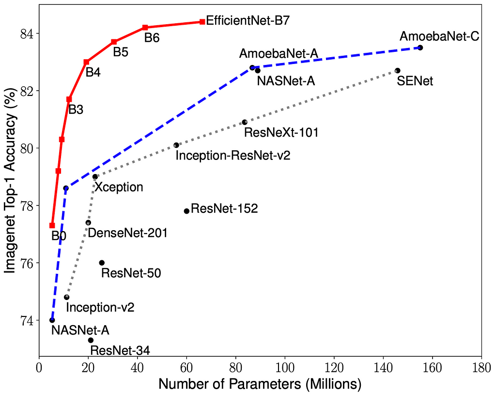
As seen from the image, even though the Top-1 Accuracy of EfficientNetB0 is comparatively low, we will be using it in this experiment to implement transfer learning, feature extraction and fine-tuning. The other higher model architectures in the EfficientNet family will require even more computationally powerful hardware.
We begin by importing the neccessary packages:
#importing the necessary packages
import tensorflow as tf
import tensorflow_datasets as tfds
import pandas as pd
import numpy as np
import matplotlib.pyplot as plt
import random
As the dataset contains 75750 train images and 25250 test images, it can be classified as a large dataset. We want to make sure, we use the GPU for computing on this large dataset as it can significantly reduce the processing, computation and training times.
print(f"The number of GPUs: {len(tf.config.list_physical_devices('GPU'))}")
!nvidia-smi -L
The number of GPUs: 1
GPU 0: NVIDIA GeForce RTX 3060 Laptop GPU (UUID: GPU-75f6c570-b9ee-76ef-47cd-a5fe65710429)
Great, my laptop’s GPU is in use.
We create the train and test datasets using the tfds.load() function. The shuffle_files parametet is set to False as we will be separately shuffling the train dataset images later while keeping the test dataset un-shuffled as we will want to compare the test set with the predicted set after evaluation on the test dataset. We also set the as_supervised parameter to True as we want a clean dataset in the ('image', 'label') format.
Note: The below step may take a long time (~1 hour) depending upon your network speed and processing power as Tensorflow downloads the whole Food101 dataset and stores it locally (about 4.65 GiB)
(train_data, test_data), ds_info = tfds.load("food101",
                                             data_dir="D:\Food Vision",
                                             split=["train", "validation"],
                                             shuffle_files=False,
                                             with_info=True,
                                             as_supervised=True)
We print the metadata information on the dataset which is saved into ds_info obtained by passing the wiht_info = True argument and get a bunch of metadata information on the dataset structure. A quick check on the number of images in the train and test datasets confirms that train dataset contains 75750 images (750 images per class) and the test dataset contains 25250 images (250 images per class) over 101 classes:
len(train_data), len(test_data)
(75750, 25250)
Calling the features method on ds_info yields the dataset structure which is currently in the form of a dictionary where the keys are image and their corresponding label. Their datatypes are uint8 and int64 respectively.
ds_info.features
FeaturesDict({
    'image': Image(shape=(None, None, 3), dtype=tf.uint8),
    'label': ClassLabel(shape=(), dtype=tf.int64, num_classes=101),
})
The class names of all the 101 food classes can be obtained by calling the names method on the label key from the dictionary. The first ten class names and the length of the list are displayed:
class_names = ds_info.features['label'].names
class_names[:10], len(class_names)
(['apple_pie',
  'baby_back_ribs',
  'baklava',
  'beef_carpaccio',
  'beef_tartare',
  'beet_salad',
  'beignets',
  'bibimbap',
  'bread_pudding',
  'breakfast_burrito'],
 101)
As EfficientNetB0 works best with images of size (224, 224, 3), it is essential that we convert all the images in our datasets to the said size. We do this by defining a function which we can later map to all the elements in the train and test datasets. Oh, and also since neural networks work best with float32 or float16 datatypes, we need to convert the uint8 datatype of the images to float32 datatype.
def resize_images(image, label):
    image = tf.image.resize(image, size=(224,224))
    image = tf.cast(image, dtype = tf.float32)
    return image, label
Now that we have defined the required function to resize the image, change the datatype and return a tuple of the image and its associated label, we will now map the created function across all elements of the dataset. At this stage, we also create a performance pipeline to fit the datasets in memory and speed up computations and processing. The num_parallel_calls parameter in the map() function is set to tf.data.AUTOTUNE which automatically tunes the mapping function to increase parallel processing efficiency. Next, we shuffle only the train dataset with a buffer size of 1000 so as to not consume a lot of memory at once and we also split the train and test datasets into batches of 32 since we cannot fit all the images in the train dataset into the GPU's bandwidth at once. We also make use of prefetch() which overlaps the preprocessing and model execution of a training step thereby increasing efficiency and decreasing the time take during training. Here too, we set the buffer_size parameter to tf.data.AUTOTUNE to let Tensorflow automatically tune the buffer size. You can read more about prefetching here.
train_data = train_data.map(map_func=resize_images, num_parallel_calls=tf.data.AUTOTUNE)
train_data = train_data.shuffle(buffer_size=1000).batch(batch_size=32).prefetch(buffer_size=tf.data.AUTOTUNE)

#test_data doesn't need to be shuffled
test_data = test_data.map(map_func=resize_images, num_parallel_calls=tf.data.AUTOTUNE)
test_data = test_data.batch(batch_size=32).prefetch(buffer_size=tf.data.AUTOTUNE)
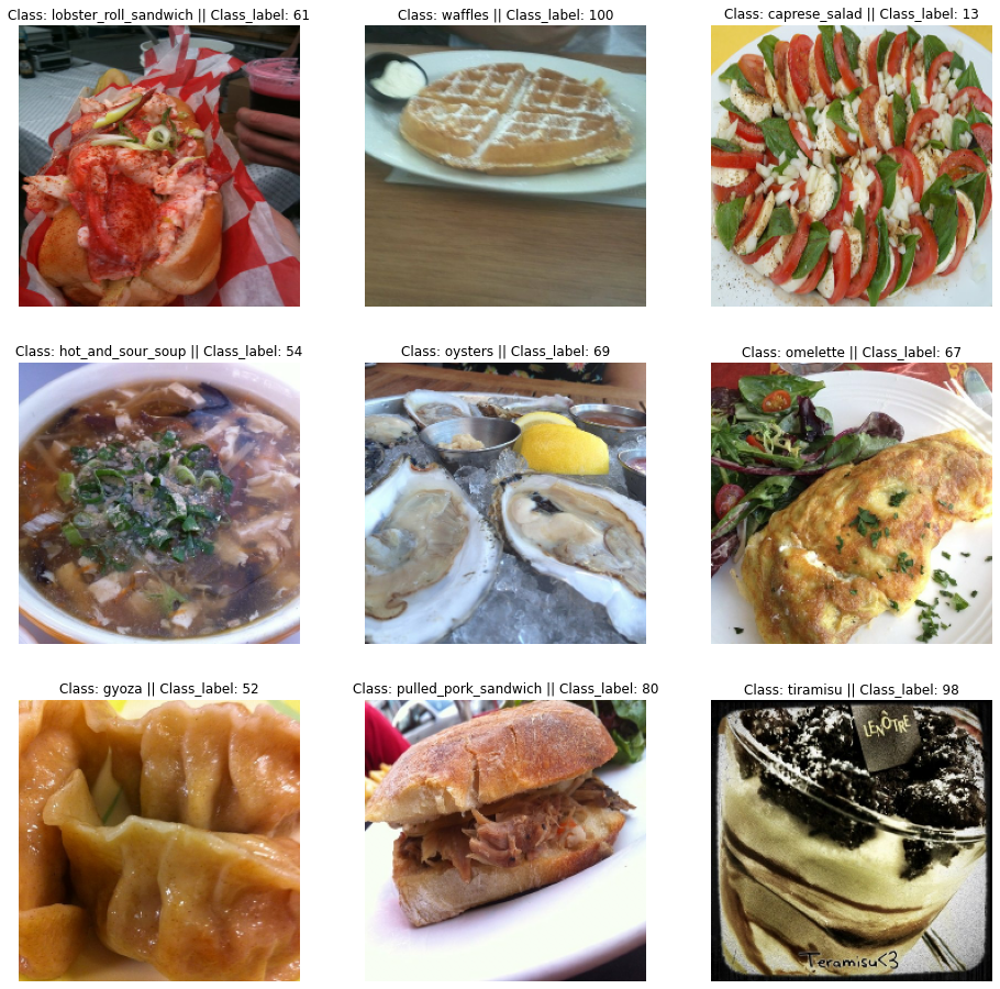
Now that we have preprocessed our train and test datasets, an important step would be to visualize the images in the dataset. We run the following code to randomly visualize 9 images across the train dataset. The image is divided by 255 as the plt.imshow() function outputs the visualization in the correct format only if all the values in the image tensor are between 0 and 1. We also print the class name and the corresponding class label of the visualized image from the train dataset:
Note: Every time this code block is run, it displays another set of random images. This is really useful to go through a few iterations and check the structure of our dataset and any labelling mistakes or other data input issues, if they occur.
plt.figure(figsize=(16,16))
for i in range(9):
    for image,label in train_data.take(1):
        image = image/255.
        plt.subplot(3,3,i+1)
        plt.imshow(image[0])
        plt.title("Class: " + class_names[label[0].numpy()] + " || Class_label: " + str(label[0].numpy()))
        plt.axis(False);
Now that we have passed the resize_images() function to our datasets to resize the images and change the datatype, we can use the element_spec attribute to check the properties of the datasets:
train_data.element_spec, test_data.element_spec
((TensorSpec(shape=(None, 224, 224, 3), dtype=tf.float32, name=None),
  TensorSpec(shape=(None,), dtype=tf.int64, name=None)),
 (TensorSpec(shape=(None, 224, 224, 3), dtype=tf.float32, name=None),
  TensorSpec(shape=(None,), dtype=tf.int64, name=None))
Great! Now all the images are of size (224, 224, 3) and the datatypes are of the float32 datatype. The None shape indicates that the images and labels have been split into batches which we specified earlier.
Oh and another thing we could do to increase our processing speed and thereby decrease the time taken to train a neural network in the process is by implementing the mixed_precision training from the keras module. Mixed precision is the use of both 16-bit and 32-bit floating-point types in a model during training to make it run faster and use less memory. The Keras mixed precision API allows us to use a mix of float16 with float32, to get the performance benefits from float16 and the numeric stability benefits from float32. You can read more about mixed_precision training here.
from tensorflow.keras import mixed_precision
mixed_precision.set_global_policy('mixed_float16')
INFO:tensorflow:Mixed precision compatibility check (mixed_float16): OK
Your GPU will likely run quickly with dtype policy mixed_float16 as it has compute capability of at least 7.0. Your GPU: NVIDIA GeForce RTX 3060 Laptop GPU, compute capability 8.6
mixed_precision.global_policy()
<Policy "mixed_float16">
We can see that the global datatype policy for our session is currenly set to mixed_float16. Also another thing to keep in mind is that, as of now, mixed precision training works only on GPUs with a compute capability of 7.0 or higher. We can see that my GPU is mixed precision training capable with a compute capability of 8.6. Thank you Nvidia!
Before we start with the actual transfer learning and fine-tuning, we will create some handy callbacks to implement during training. The first will be the TensorBoard callback which can produce well-deinfed graphs and visualizations of our model's metrics on the Tensorboard Dev site. To do this, we simply provide a path to store the callback during training.
Secondly, we will create a ModelCheckpoint callback which will create a checkpoint of our model which we can later revert back to, if needed. Here we save only the weights of the model and not the whole model itself as it can take some time. The validation accuracy is the metric being monitored here and we also set the save_best_only parameter to True and so the callback will only the save the weights of the model which has led to the highest validation accuracy.
def tensorboard_callback(directory, name):
    log_dir = directory + "/" + name
    t_c = tf.keras.callbacks.TensorBoard(log_dir = log_dir)
    return t_c

def model_checkpoint(directory, name):
    log_dir = directory + "/" + name
    m_c = tf.keras.callbacks.ModelCheckpoint(filepath=log_dir,
                                             monitor="val_accuracy",
                                             save_best_only=True,
                                             save_weights_only=True,
                                             verbose=1)
    return m_c
Okay now that we have preprocessed our data, visualized and created some handy callbacks, we move on the the acutal transfer learning part! We create the base model with tf.keras.applications.efficientnet and choose EfficientNetB0 from the list of available EfficientNet prebuilt models. We also set the include_top parameter to False as we will be using our own output classifier layer suited to our food101 classification application. Since we are just feature extracting and not fine-tuning at this point, we will set base_model.trainable = False.
base_model = tf.keras.applications.efficientnet.EfficientNetB0(include_top=False)
base_model.trainable = False
Now that we have our feature extraction base model ready, we will use the Keras Functional API to create our model which include the base model as functional layer for our feature extraction training model. The input layer is first created with the shape set to (224, 224, 3). The base model layer is then instantiated by passing the input layer while also setting the training parameter to False as we are not into fine-tuning the model yet. Next, the GlobalAveragePooling2D layer is set up to perform the pooling operation for our convolutional neural network. After that, a small change is done where this model differs from the conventional CNN, where the output layer is split separately into the Dense and Activation layers. Usually for any classification, the softmax activation can be included along with the output Dense layer. But here, since we have implemented mixed_precision training, we pass the Activation layer separately at the end as we want the output from the softmax activation to be of the float32 datatype which will rid us of any stability errors by maintaining numeric stability. Finally, the model is created by using the Model() function.
from tensorflow.keras import layers

inputs = layers.Input(shape = (224,224,3), name='inputLayer')
x = base_model(inputs, training = False)
x = layers.GlobalAveragePooling2D(name='poolingLayer')(x)
x = layers.Dense(101, name='outputLayer')(x)
outputs = layers.Activation(activation="softmax", dtype=tf.float32, name='activationLayer')(x)

model = tf.keras.Model(inputs, outputs, name = "FeatureExtractionModel")
Now that we have built the model with just feature extraction included, we use the summary() method to get a look at the architecture of our feature extraction model:
model.summary()
Model: "FeatureExtractionModel"
_________________________________________________________________
Layer (type)                 Output Shape              Param #
=================================================================
inputLayer (InputLayer)      [(None, 224, 224, 3)]     0
_________________________________________________________________
efficientnetb0 (Functional)  (None, None, None, 1280)  4049571
_________________________________________________________________
poolingLayer (GlobalAverageP (None, 1280)              0
_________________________________________________________________
outputLayer (Dense)          (None, 101)               129381
_________________________________________________________________
activationLayer (Activation) (None, 101)               0
=================================================================
Total params: 4,178,952
Trainable params: 129,381
Non-trainable params: 4,049,571
_________________________________________________________________
We see that the whole base model (EfficientNetB0) is implemented as a single functional layer in our feature extraction model. We also see the other layers created for building our model. The base model contains about 4 million parameters but they are all non-trainable since we have frozen the base model as we are not fine tuning but rather only extracting the features from the base model. The only trainable parameters come from the output Dense layer.
Next, we get a detailed look at the various layers in our feature extraction model, their names, see if they are trainable or not, their data types and their corresponding data type policies.
for lnum, layer in enumerate(model.layers):
    print(lnum, layer.name, layer.trainable, layer.dtype, layer.dtype_policy)
0 inputLayer True float32 <Policy "float32">
1 efficientnetb0 False float32 <Policy "mixed_float16">
2 poolingLayer True float32 <Policy "mixed_float16">
3 outputLayer True float32 <Policy "mixed_float16">
4 activationLayer True float32 <Policy "float32">
We can see that all the layers excepting the base model layer are trainable. The datatype policies indicate that apart from the input layer and the output activation layer which have float32 datatype policy, all the other layers are compatible with and employ the mixed_float16 datatype policy.
Now we can move on to compiling and fitting our model. Since our labels are not one-hot encoded, we use the SparseCategoricalCrossentropy() loss function. We use the Adam() optimizer with its default learning rate and set the model metrics to measure accuracy.
Then we begin to fit our feature extraction model. We save the model fitting history variable into hist_model and we train our model on the train dataset for 3 epochs. We use our test dataset as the validation data while training and use 10% of the test data as the validation step count to decrease the time taken for each epoch. We also pass the previously created callback functions into the callbacks list to create a TensorBoard Dev visualization and also a ModelCheckpoint which saves our model's best weights while monitoring the validation accuracy.
model.compile(loss = tf.keras.losses.SparseCategoricalCrossentropy(),
              optimizer = tf.keras.optimizers.Adam(),
              metrics = ["accuracy"])

hist_model = model.fit(train_data,
                       epochs = 3,
                       steps_per_epoch=len(train_data),
                       validation_data=test_data,
                       validation_steps=int(0.1 * len(test_data)),
                       callbacks=[tensorboard_callback("Tensorboard","model"),                                  model_checkpoint("Checkpoints","model.ckpt")])
Epoch 1/3
2368/2368 [==============================] - 115s 43ms/step - loss: 1.8228 - accuracy: 0.5578 - val_loss: 1.2524 - val_accuracy: 0.6665

Epoch 00001: val_accuracy improved from -inf to 0.66653, saving model to Checkpoints\model.ckpt
Epoch 2/3
2368/2368 [==============================] - 97s 41ms/step - loss: 1.2952 - accuracy: 0.6656 - val_loss: 1.1330 - val_accuracy: 0.6946

Epoch 00002: val_accuracy improved from 0.66653 to 0.69462, saving model to Checkpoints\model.ckpt
Epoch 3/3
2368/2368 [==============================] - 100s 42ms/step - loss: 1.1449 - accuracy: 0.7024 - val_loss: 1.0945 - val_accuracy: 0.7021

Epoch 00003: val_accuracy improved from 0.69462 to 0.70214, saving model to Checkpoints\model.ckpt
Wow! I was expecting the training time for each epoch to take a lot longer. It seems like our input data pipelining, GPU and the mixed_precision policy implementation have really helped us reduce the time take for training significantly.
Hmm… our training and validation accuracies are not that bad considering we have 101 output classes. We have also created a model checkpoint with the model weights leading to the highest validation accuracy incase we want to revert back to it after fine-tuning in the next stage. Let us evaluate our model on the whole test data now and store it in a variable.
model_results = model.evaluate(test_data)
790/790 [==============================] - 27s 34ms/step - loss: 1.0932 - accuracy: 0.7053
Not bad, not bad at all. 70.53% accuracy is pretty decent for just a feature extraction model.
We have got an accuracy of about 70.53% with our feature extraction model based on the EfficientNetB0 base model. How about we try to increase the accuracy score by fine-tuning our feature extraction model now. To do this, we set the layers of our model’s base_model (the EfficientNetB0 functional layer) to be trainable and unfreeze the previously frozen base model.
base_model.trainable = True
However, The BatchNormalization layers need to be kept frozen. If they are also turned to trainable, the first epoch after unfreezing will significantly reduce accuracy (details here). Since all the layers in the base model have been set to trainable, we use the following code block to again freeze only the BatchNormalization layers of our base model:
for layer in model.layers[1].layers:
    if isinstance(layer, layers.BatchNormalization):
        layer.trainable = False
A quick check on the base model’s layers, their datatypes and policies and whether or not they’re trainable:
for lnum, layer in enumerate(model.layers[1].layers[-10:]):
    print(lnum, layer.name, layer.trainable, layer.dtype, layer.dtype_policy)
0 block6d_project_conv True float32 <Policy "mixed_float16">
1 block6d_project_bn False float32 <Policy "mixed_float16">
2 block6d_drop True float32 <Policy "mixed_float16">
3 block6d_add True float32 <Policy "mixed_float16">
4 block7a_expand_conv True float32 <Policy "mixed_float16">
5 block7a_expand_bn False float32 <Policy "mixed_float16">
6 block7a_expand_activation True float32 <Policy "mixed_float16">
7 block7a_dwconv True float32 <Policy "mixed_float16">
8 block7a_bn False float32 <Policy "mixed_float16">
9 block7a_activation True float32 <Policy "mixed_float16">
Good! Looks like all the layers in the base model are trainable and ready for fine tuning except for the BatchNormalization layers. I think we are good to proceed and fine tune our feature extraction model 'model'. We begin by compiling the model again since we have change the layer attributes (unfreeze), but this time, as a general good practice, we reduce the default learning rate of the Adam() optimizer by ten times so as to reduce overfitting and stop the model from learning/memorizing the train data to a great extent.
Then we begin to fit our fine tuning model. We save the model fitting history variable into hist_model_tuned and we train our model on the train dataset for 5 epochs, however, we set the initial epoch to be the last epoch from our feature extraction model training which would be 3. Thus the fine tuning model training would start from epoch number 3 and would run upto 5 (three epochs total). We use our test dataset as the validation data while training and use 10% of the test data as the validation step count to decrease the time taken for each epoch. We again pass the previously created callback functions into the callbacks list to create a TensorBoard Dev visualization for comparison between the feature extraction and this fine tuning models and also a ModelCheckpoint which saves our model's best weights while monitoring the validation accuracy.
model.compile(loss = tf.keras.losses.SparseCategoricalCrossentropy(),
              optimizer = tf.keras.optimizers.Adam(learning_rate=0.0001),
              metrics = ["accuracy"])
hist_model_tuned = model.fit(train_data,
                             epochs=5,
                             steps_per_epoch=len(train_data),
                             validation_data=test_data,
                             validation_steps=int(0.1*len(test_data)),
                             initial_epoch=hist_model.epoch[-1],
                             callbacks=[tensorboard_callback("Tensorboard", "model_tuned"), model_checkpoint("Checkpoints", "model_tuned.ckpt")])
Epoch 3/5
2368/2368 [==============================] - 313s 127ms/step - loss: 0.9206 - accuracy: 0.7529 - val_loss: 0.8053 - val_accuracy: 0.7757

Epoch 00003: val_accuracy improved from -inf to 0.77571, saving model to Checkpoints\model_tuned.ckpt
Epoch 4/5
2368/2368 [==============================] - 297s 125ms/step - loss: 0.5628 - accuracy: 0.8457 - val_loss: 0.8529 - val_accuracy: 0.7678

Epoch 00004: val_accuracy did not improve from 0.77571
Epoch 5/5
2368/2368 [==============================] - 298s 125ms/step - loss: 0.3082 - accuracy: 0.9132 - val_loss: 0.8977 - val_accuracy: 0.7801

Epoch 00005: val_accuracy improved from 0.77571 to 0.78006, saving model to Checkpoints\model_tuned.ckpt
Okay great! Looks like the validation accuracy has improved a lot. Let’s evaluate our fine-tuned model on the whole test data now and store it in a variable.
model_tuned_results = model.evaluate(test_data)
790/790 [==============================] - 26s 33ms/step - loss: 0.9043 - accuracy: 0.7772
Would you look at that! The fine-tuned model’s accuracy has improved by about 10% and is now at about 77.72%. That is a huge increase we have achieved with just transfer learning and fine-tuning. Thanks EfficientNet for your model!
As a comparison, Deep Food’s Convolutional Neural Network model implemented back in June of 2016 had achieved a Top-1 Accuracy of 77.4%. Deep Food’s CNN model took days to train whereas our transfer learning applied model was built just under 15 minutes! Moreover, our model is almost on par with it or slightly better even just by using simple transfer learning techniques and fine tuning. Training for more epochs and adding regularization techniques to reduce overfitting among other methods can surely improve our fine tuned model’s accuracy score. We could also save our model to a directory at this point using the .save() function to use it outside of our local runtime.
Since we have created TensorBoard callbacks, we can upload the saved TensorBoard logs in the specified directory to TensorBoard Dev. The obtained link can be clicked to view the model's metric visualizations online in TensorBoard Dev.
!tensorboard dev upload --logdir ./Tensorboard \
 --name "Food101"\
 --description "Feature Extraction Model vs Fine Tuned Model"\
 --one_shot
New experiment created. View your TensorBoard at: https://tensorboard.dev/experiment/hveaY1MSQBK6wIN6MwXoHA/

[2021-11-16T23:06:17] Started scanning logdir.
Data upload starting...
Uploading binary object (884.4 kB)...
Uploading binary object (1.1 MB)...
Uploading 36 scalars...
[2021-11-16T23:06:22] Total uploaded: 36 scalars, 0 tensors, 2 binary objects (2.0 MB)
[2021-11-16T23:06:22] Done scanning logdir.


Done. View your TensorBoard at https://tensorboard.dev/experiment/hveaY1MSQBK6wIN6MwXoHA/
Since we have created two history objects for both the feature extraction model and the fine-tuned model, we can create a function to plot both the histories together and compare the training and the validation metrics to get a general idea of the performance of both models:
def compare_histories(original_history, new_history, initial_epochs):
    """
    Compares two model history objects.
    """
    acc = original_history.history["accuracy"]
    loss = original_history.history["loss"]

    val_acc = original_history.history["val_accuracy"]
    val_loss = original_history.history["val_loss"]

    total_acc = acc + new_history.history["accuracy"]
    total_loss = loss + new_history.history["loss"]

    total_val_acc = val_acc + new_history.history["val_accuracy"]
    total_val_loss = val_loss + new_history.history["val_loss"]

    plt.figure(figsize=(9, 9))
    plt.subplot(2, 1, 1)
    plt.plot(total_acc, label='Training Accuracy')
    plt.plot(total_val_acc, label='Validation Accuracy')
    plt.plot([initial_epochs-1, initial_epochs-1],
              plt.ylim(), label='Start of Fine Tuning')
    plt.legend(loc='lower right')
    plt.title('Training and Validation Accuracy')

    plt.subplot(2, 1, 2)
    plt.plot(total_loss, label='Training Loss')
    plt.plot(total_val_loss, label='Validation Loss')
    plt.plot([initial_epochs-1, initial_epochs-1],
              plt.ylim(), label='Start of Fine Tuning')
    plt.legend(loc='upper right')
    plt.title('Training and Validation Loss')
    plt.xlabel('epoch')
    plt.show()
Great! Now let us use both the hist_model and hist_model_tuned objects along the function with the initial_epochs set to 3 since we trained our first feature extraction model for 3 epochs.
compare_histories(hist_model, hist_model_tuned, initial_epochs=3)
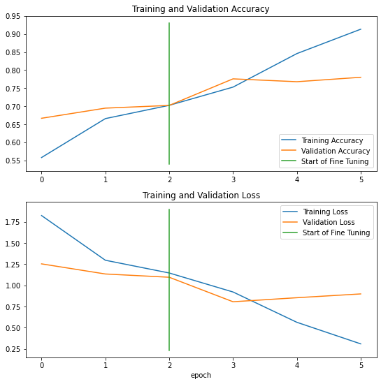
Hmm… that is a good plot. The training and validation curves look good for the feature extraction model, however, after fine-tuning, after just one epoch, the training loss decreases significantly while the training accuracy increases sharply. All this time, the validation accuracy and loss begin to plateau. This surely denotes that our model is over-fitting after an epoch. Other regularization techniques including drop-outs, augmentation and Early-Stopping callback techniques can be used to reduce over-fitting and maybe improve our model’s accuracy scores on unseen test data. However, we will not be exploring them now as this experiment was just to showcase the incredible power of transfer learning and fine-tuning with just a few easy steps.
Now that we have trained our fine-tuned model based on EfficientNetB0, we will use it to make predictions on the whole test dataset and store it in preds:
preds = model.predict(test_data, verbose = 1)
790/790 [==============================] - 27s 32ms/step
Note: The predictions are stored in a collection of prediction probabilities for each class for an individual test image.
Now that we have the prediction probabilities for each class for a given test image, we can easily obtain the prediction labels using the tf.argmax() function which returns the index which contains the highest probability along a given axis. We store the prediction labels in pred_labels:
pred_labels = tf.argmax(preds, axis=1)
pred_labels[:10]
<tf.Tensor: shape=(10,), dtype=int64, numpy=array([ 29, 81, 91, 53, 97, 97, 10, 31, 3, 100], dtype=int64)>
Now that we have made predictions and obtained the prediction labels, we can compare it with the test dataset labels to get detailed information on how well the fine-tuned model has made its predictions. We get the test labels from the test dataset using the following code block employing list comprehension:
test_labels = np.concatenate([y for x, y in test_data], axis=0)
test_labels[:10]
array([ 29, 81, 91, 53, 97, 97, 10, 31, 3, 100], dtype=int64)
Great! We now have both the predicted labels and the ground truth test labels. However to plot our prediction labels along with the associated image, we will need a dataset containing only the images extracted from test_data which contains both the images along with the labels. To do this, two steps are needed. First, we create an empty list and pass a for loop which extracts and appends each batch from the test dataset using the take() function to the newly created empty list test_image_batches. The -1 inside the take() function makes the for loop to pass through all the batches in the test data. The resulting output is a list of all the batches in the test data. Since the images are still in batches in the form of sublists inside the list test_image_batches, in step 2, we use list comprehension to extract each sublist, i.e each image from the main list and store them in the test_images list. The resulting list test_images contains all the 25250 test images contained in the original test dataset which is verified by using the len() funtion on the list.
# Step 1
test_image_batches = []
for images, labels in test_data.take(-1):
    test_image_batches.append(images.numpy())

# Step 2
test_images = [item for sublist in test_image_batches for item in sublist]
len(test_images)
25250
Now that we have a list of test images(test_images), their ground truth test labels(test_labels) and their corresponding prediction labels(pred_labels) along with the prediction probabilities (preds), we can easily visualize the test images along with their predictions including the ground truth and prediction class names.
Here, we take 9 random images from test_images and plot them along with the ground truth class names and predicted class names in the plot title, side by side using indexing on class_names with the corresponding ground truth and predicted labels. We also display the prediction probabilities of the predictions on each image to get an idea of how confident the model is in its predictions. Moreover, to make the plots looke good and more informative, for wrong predictions, we set the title color to red, whereas for correct predictions by our fine-tuning model, we set the title color to green.
Note: Each time this code block is run, it display a new random set of images and their predictions, this can be particularly useful in identifying two similar looking food classes where our model might get confused or an instance where our model has correctly predicted an image but it falls into the wrongly predicted category because of a wrong ground truth test label.
plt.figure(figsize = (20,20))
for i in range(9):
    random_int_index = random.choice(range(len(test_images)))
    plt.subplot(3,3,i+1)
    plt.imshow(test_images[random_int_index]/255.)
    if test_labels[random_int_index] == pred_labels[random_int_index]:
        color = "g"
    else:
        color = "r"
    plt.title("True Label: " + class_names[test_labels[random_int_index]] + " || " + "Predicted Label: " +
              class_names[pred_labels[random_int_index]] + "\n" +
              str(np.asarray(tf.reduce_max(preds, axis = 1))[random_int_index]), c=color)
    plt.axis(False);

As we have both the test and prediction labels, we can also use the classification_report() function from SciKit-Learn library and store the precision, recall and f1-scores for each class in a dictionary report by specifying the output_dict parameter to be True.
from sklearn.metrics import classification_report
report = classification_report(test_labels, pred_labels, output_dict=True)

#check a small slice of the dictionary
import itertools
dict(itertools.islice(report.items(), 3))
{'0': {'precision': 0.5535055350553506,
  'recall': 0.6,
  'f1-score': 0.5758157389635316,
  'support': 250},
 '1': {'precision': 0.8383838383838383,
  'recall': 0.664,
  'f1-score': 0.7410714285714286,
  'support': 250},
 '2': {'precision': 0.9023255813953488,
  'recall': 0.776,
  'f1-score': 0.8344086021505377,
  'support': 250}}
Now that we have a dictionary containing the various evaluation metrics (precision, recall and f1-scores), how about we create a pandas dataframe which contains only the class names along with its corresponding F1-score. We choose the F1-score among the evaluation metrics as it achieves a balance between the precision and recall. You can read more about evaluation metrics here.
However, in order to create that required dataframe, we will need to extract the class labels(keys) and the corresponding F1-score(part of values) from the classification report dictionary. This can be achieved by creating an empty dictionary f1scores and passing a for loop which goes through the original dictionary report's items(keys and values) and appends the class names using key-indexing and the corresponding F1-score by value-indexing.
f1scores = {}
for k,v in report.items():
    if k == 'accuracy':
        break
    else:
        f1scores[class_names[int(k)]] = v['f1-score']

#check a small slice of the dictionary
dict(itertools.islice(f1scores.items(), 5))
{'apple_pie': 0.5758157389635316,
 'baby_back_ribs': 0.7410714285714286,
 'baklava': 0.8344086021505377,
 'beef_carpaccio': 0.7912087912087912,
 'beef_tartare': 0.7118644067796612}
Now that we have the required dictionary ready, we can easily create a dataframe F1 form the following line of code and sort the dataframe by the descending order of the various classes' F1-scores:
F1 = pd.DataFrame({"Classes":list(f1scores.keys()),
                   "F1-Scores":list(f1scores.values())}).sort_values("F1-Scores", ascending=False)

#check a small slice of the dataframe
F1[:10]
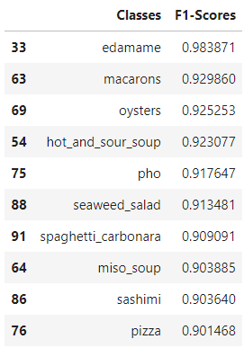
Great! It seems like the food class edamame has achieved the highest F1-score among all the classes followed by macarons. What's stopping us from creating a neat bar chart visualization displaying all the 101 food classes and their F1-scores in a descending order?
fig, ax = plt.subplots(figsize = (15,20))
plt.barh(F1["Classes"], F1["F1-Scores"])
plt.ylim(-1,101)
plt.xlabel("F1-Scores")
plt.ylabel("Food Classes")
plt.title("F1-Scores across various Food Classes")
plt.gca().invert_yaxis()
for i, v in enumerate(round(F1["F1-Scores"],3)):
    ax.text(v, i + .25, str(v), color='red');
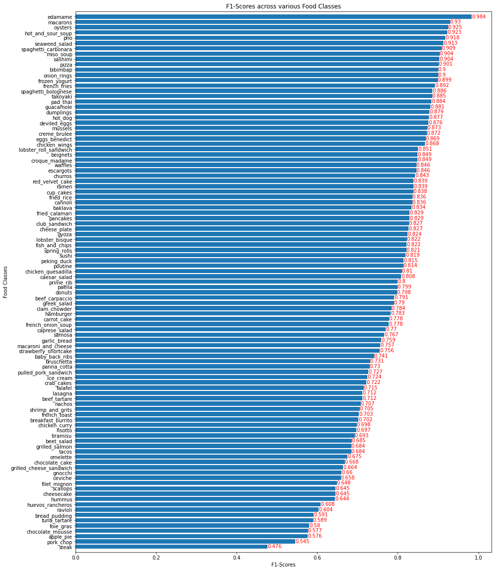

Fantastic! The food class edamame has the highest number of correct predictions while the class steak has the lowest F1-score, by far, indicating the lowest number of correct predictions. Hmm.. that's kinda sad because we all love steak!
As a final evaluation step for our transfer learning fine-tuned model based on the EfficientNetB0 let’s visualize the most wrong predictions of our model, i.e the false(wrong) predictions of our model where the prediction probability is the highest. This will help us get an idea about our model as to whether it is getting confused on similar food classes or whether a test image has been wrongly labelled which would be a data input error.
To do this, let’ss create a neat dataframe Predictions which contains the 'Image Index' of the various images in the test dataset, their corresponding 'Test Labels', 'Test Classes', 'Prediction Labels', 'Prediction Classes', and 'Prediction Probability'.
Predictions = pd.DataFrame({"Image Index" : list(range(25250)),
                            "Test Labels" : list(test_labels),
                            "Test Classes" : [class_names[i] for i in test_labels],
                            "Prediction Labels" : list(np.asarray(pred_labels)),
                            "Prediction Classes" : [class_names[i] for i in pred_labels],
                            "Prediction Probability" : [x for x in np.asarray(tf.reduce_max(preds, axis = 1))]})
As we have created the required dataframe Predictions, we can also create a new column 'Correct Prediction' which contains True for test images that have been correctly predicted by our model and False for wrongly predicted test images:
Predictions["Correct Prediction"] = Predictions["Test Labels"] == Predictions["Prediction Labels"]
Predictions[:10]
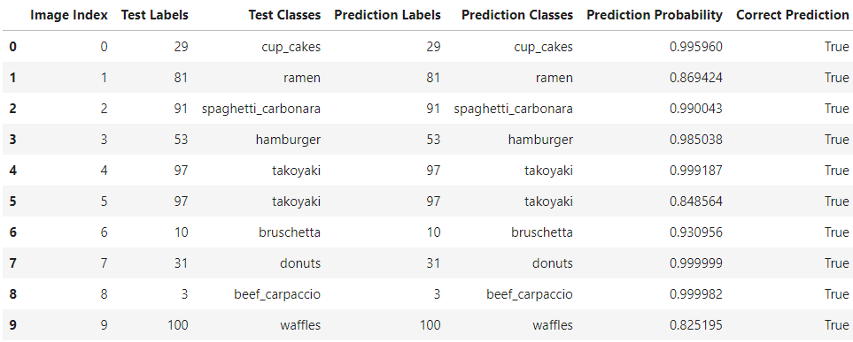
Great, our dataframe looks fantastic! However, this is not the final form of our dataframe. We want to subset our current dataframe with only those records where ‘Correct Prediction’ is equal to False as our aim is to plot and visualize the most wrong predictions of our fine-tuning model. We obtain our final dataframe using the following code block and sort the dataframe records in the descending order of the 'Prediction Probability':
Predictions = Predictions[Predictions["Correct Prediction"] == False].sort_values("Prediction Probability", ascending=False)
Predictions[:10]
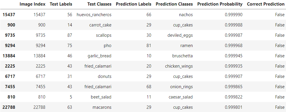
Impressive! Our final dataframe Predictions contains only the wrongly predicted image records (image indexes) along with their ground truth test labels, test classes, predicted labels, prediction classes sorted by the descending order of their prediction probabilities. We can manually take an image index out of this dataset and pass it into a plot function on the test dataset to obtain a visualization of the image with its ground truth class name and the predicted class name. However, here we will take the first 9 images or image indexes which are the most wrong images in our dataframe and plot it along with the true class names, the predicted class names and the corresponding prediction probabilities.
indexes = np.asarray(Predictions["Image Index"][:9]) #choosing the top 9 records from the dataframe
plt.figure(figsize=(20,20))
for i, x in enumerate(indexes):
    plt.subplot(3,3,i+1)
    plt.imshow(test_images[x]/255)
    plt.title("True Class: " + class_names[test_labels[x]] + " || " + "Predicted Class: " + class_names[pred_labels[x]] + "\n" +
             "Prediction Probability: " + str(np.asarray(tf.reduce_max(preds, axis = 1))[x]))
    plt.axis(False);

Well well well… what do you know! Through quick Google searches (yes, I don’t know what most of these food class names are), it becomes pretty evident that in fact, the ground truth test labels for some test images have been wrongly labelled as in the case of the first image which is clearly not huevos rancheros but is indeed the class predicted by our model — nachos! Also, the fith image is clearly not garlic bread but is also the class predicted by our model — bruschetta! Extra points to our model! Other common wrong predictions arise from our model getting confused between similar looking food classes. For example the chocolate_cake in some images closely resembles tiramisu and in some cases would be really hard for even a human being to classify.
Good thing we decided to visualize the most wrong predictions! With this, we can perform appropriate data cleaning techniques to correct the wrong truth labels and maybe remove some really confusing similar looking food classes. After performing these corrections and adjustments, I think our fine-tuned model’s accuracy can be increased drastically!
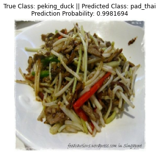
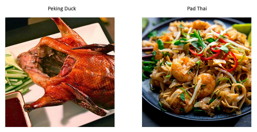
Again, while randomly going through the most wrong predicted images, I came across this image which is clearly true labelled peking_duck in the test dataset but is indeed pad_thai! Once more, this can be confirmed by a quick Google search and thus our model has actually made the correct prediction. Hmm... maybe many other images with wrong ground truth labels exist and if all of them are corrected, imagine our model's accuracy score!
plt.figure(figsize=(5,5))
plt.imshow(test_images[11586]/255)
plt.title("True Class: " + class_names[test_labels[11586]] + " || " + "Predicted Class: " + class_names[pred_labels[11586]]
          + "\n" + "Prediction Probability: " + str(np.asarray(tf.reduce_max(preds, axis = 1))[11586]))
plt.axis(False);
Now imagine if we had to build a complex model with more than two-hundred layers such as the EfficientNetB0 for our image classification tasks and to achieve this level of accuracy, how many days would it take us? Transfer learning is indeed an amazing technique!
Thank you for reading.
If you like my work, you can connect with me on Linkedin.
Image Classification Transfer Learning and Fine Tuning using TensorFlow was originally published in Towards Data Science on Medium, where people are continuing the conversation by highlighting and responding to this story.
from Towards Data Science - Medium https://ift.tt/3cmrOug
via RiYo Analytics


ليست هناك تعليقات