https://ift.tt/3jYsh9X And how these metrics change in different scenarios Image by Author Table of Contents - Accuracy - The Confusio...
And how these metrics change in different scenarios

Table of Contents
- Accuracy
- The Confusion Matrix
- A multi-label classification example
- Multilabel classification confusion matrix
- Aggregate metrics
- Some Common Scenarios
Introduction
Classification is an important application of machine learning, which involves applying algorithms that learn from data.
Classification is a predictive modelling task that requires assigning a class label to a data point, and we can say that that datapoint was classified as belonging to a particular class.
Accuracy
Developing and applying models is one thing, but without a way to evaluate them, experimentation quickly becomes pointless.
Most people know what accuracy is, even if it's just in an intuitive sense — how accurate something refers to how often it achieves some goal. That goal could be scoring in sports. When it comes to classification, it's measured by how often a model correctly classifies data.
Simply put, for a classification problem, accuracy can be measured as:
accuracy = number of correct predictions / total predictions
Accuracy doesn’t tell the whole story
This seems like a good way to evaluate a model — you’d expect a “better” model to be more accurate than some “less good” model. And while that’s generally true, accuracy sometimes fails to give you the entire picture, like imbalanced datasets, for example.
Let’s say you have data belonging to two classes: red and blue. Class red has the majority of data points. Let’s say that their proportion is 9:1.

That would mean that given 100 data points, 90 would belong to class red, while only 10 would belong to class blue.
Now, what if my model is so poorly trained that it always predicts class red, no matter what datapoint it's given?
You can probably see where I’m going with this.
In the above case, my model’s accuracy would end up being 90%. It would get all reds correct, and all blues wrong. So, accuracy would be 90 / (90 + 10) or 90%.
Objectively speaking, this would be a pretty decent classification accuracy to aim for. But accuracy, in this case, hides the fact that our model has, in fact, learned nothing at all and always predicts class red.
The Confusion Matrix
A confusion matrix is a matrix that breaks down correctly and incorrectly classified into:
- True positive (TP): Correctly predicting the positive class
- True Negative (TN): Correctly predicting the negative class
- False Positive (FP): Incorrectly predicting the positive class
- False Negative (FN): Incorrectly predicting the negative class
Using these, metrics like precision, recall and f1-score are defined, which, compared to accuracy, give us a more accurate (hah!) measure of what’s going on.
Coming back to our example, our negative class is class red and the positive class is blue. Let’s say we test our model on 100 data points. Maintaining the same distribution, 90 of the data points would be red, while 10 would be blue.
Its confusion matrix would be:
True positive   = 0
True negative   = 90
False positive  = 10
False Negative  = 0
Computing Precision, recall and F1-score
Precision = TP / (TP + FP)
          = 0 / (0 + 10)
          = 0
Recall    = TP / (TP + TN)
          = 0 / (0 + 90)
          = 0
So though my model’s accuracy was 90%, a generally good score, its precision and recall are 0, showing that the model didn’t predict the positive class even a single time.
This is a good example of where accuracy doesn’t give us the entire picture. The same is true for precision and recall individually.
Multilabel Classification
Multilabel classification refers to the case where a data point can be assigned to more than one class, and there are many classes available.
This is not the same as multi-class classification, which is where each data point can only be assigned to one class, irrespective of the actual number of possible classes.
Unlike in multi-class classification, in multilabel classification, the classes aren’t mutually exclusive
Evaluating a binary classifier using metrics like precision, recall and f1-score is pretty straightforward, so I won’t be discussing that. Doing the same for multi-label classification isn’t exactly too difficult either— just a little more involved.
To make it easier, let’s walk through a simple example, which we’ll tweak as we go along.
An Example
Let’s say we have data spread across three classes — class A, class B and class C. Our model attempts to classify data points into these classes. This is a multi-label classification problem, so these classes aren’t exclusive.
Evaluation
Let’s take 3 data points as our test set to simply things.
expected   predicted
A, C        A, B
C           C
A, B, C     B, C
We’ll first see what a confusion matrix looks like for a multilabel problem and then create a separate one for one of the classes as an example.
We’ll encode the classes A, B and C using sklearn’s MultiLabelBinarizer. So every prediction can be expressed as a three-bit string, where the first bit represents A, then B and the last bit is C.
expected    predicted
1 0 1       1 1 0
0 0 1       0 0 1
1 1 1       0 1 1
Let’s find the confusion matrix for class A based on our test.
Class A
For calculating true positive, we’re looking at the cases where our model predicted the label A and the expected labels also contained A.
So TP would be equal to 1.
Coming to FP, we are looking for those cases where our model predicted the label A but A isn’t in the true label.
So FP is 0.
Coming to TN, this is where neither the expected labels nor the predicted labels contain class A.
So TN is 1.
Finally, FN is where the A is an expected label, but it wasn’t predicted by our model.
So FN is 1.
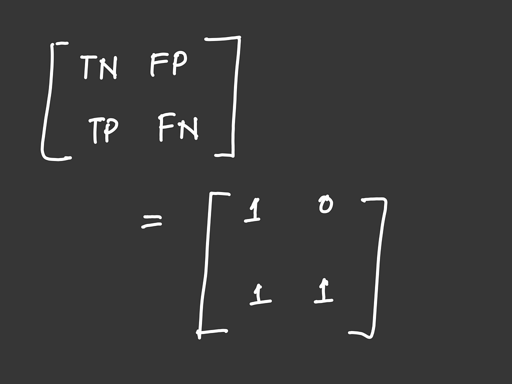
Let’s make the confusion matrix for class A using these values:
TN FP
FN TP
We get:
A similar computation can be done for the other two classes.
Class B: 1   1
         0   1
Class C: 0   0
         1   2
Confusion Matrix
Confusion matrices like the ones we just calculated can be generated using sklearn’s multilabel_confusion_matrix. We simply pass in the expected and predicted labels (after binarizing them)and get the first element from the list of confusion matrices — one for each class.
confusion_matrix_A
    = multilabel_confusion_matrix(y_expected, y_pred)[0]
The output is consistent with our calculations.
print(confusion_matrix_A)
# prints:
1  0
1  1
Precision, Recall and F1-score
Using the confusion matrices we just computed, let’s calculate each metric for class A as an example.
Precision for class A
Precision is simply:
Precision = TP / (TP + FP)
In the case of class A, that ends up being:
1 / (1 + 0) = 1
Recall for class A
Using the formula for recall given as:
Recall = TP / (TP + TN)
we get:
1 / (1 + 1) = 0.5
F1-score for class A
This is just the harmonic mean of the precision and recall we calculated.

which gives us:

These metrics can be calculated for classes B and C in the same way.
On finishing it for all the other classes, we end up with the following results:
Class B
Precision = 0.5
Recall = 1.0
F1-score = 0.667
Class C
Precision = 1.0
Recall = 0.667
F1-score = 0.8
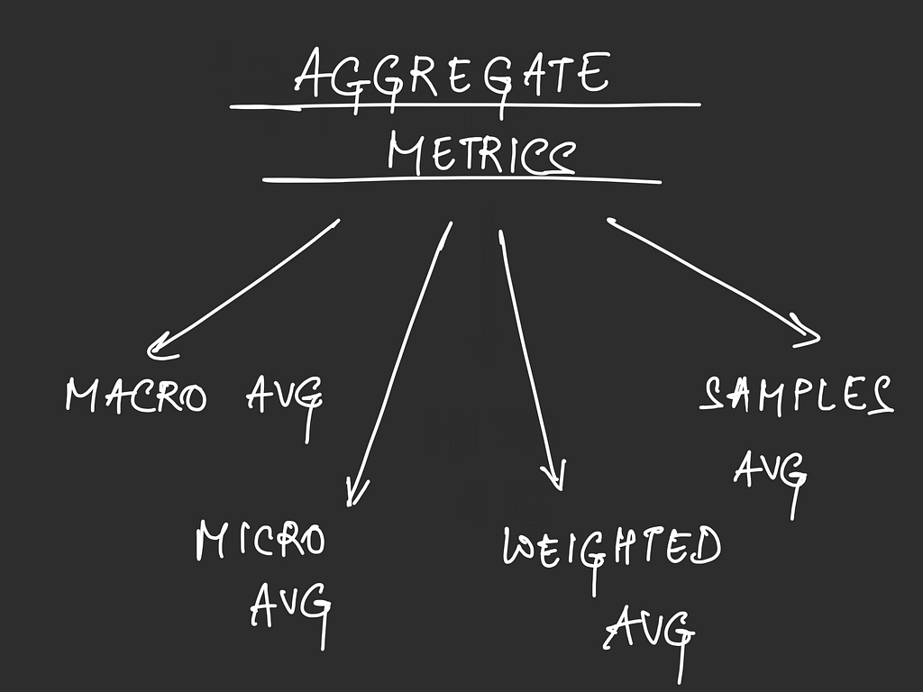
Aggregate metrics
Aggregate metrics like macro, micro, weighted and sampled avg give us a high-level view of how our model is performing.
Macro average
This is simply the average of a metric — precision, recall or f1-score — over all classes.
So in our case, the macro-average for precision would be
Precision (micro avg)
= (Precision of A + Precision of B + Precision of C) / 3
= 0.833
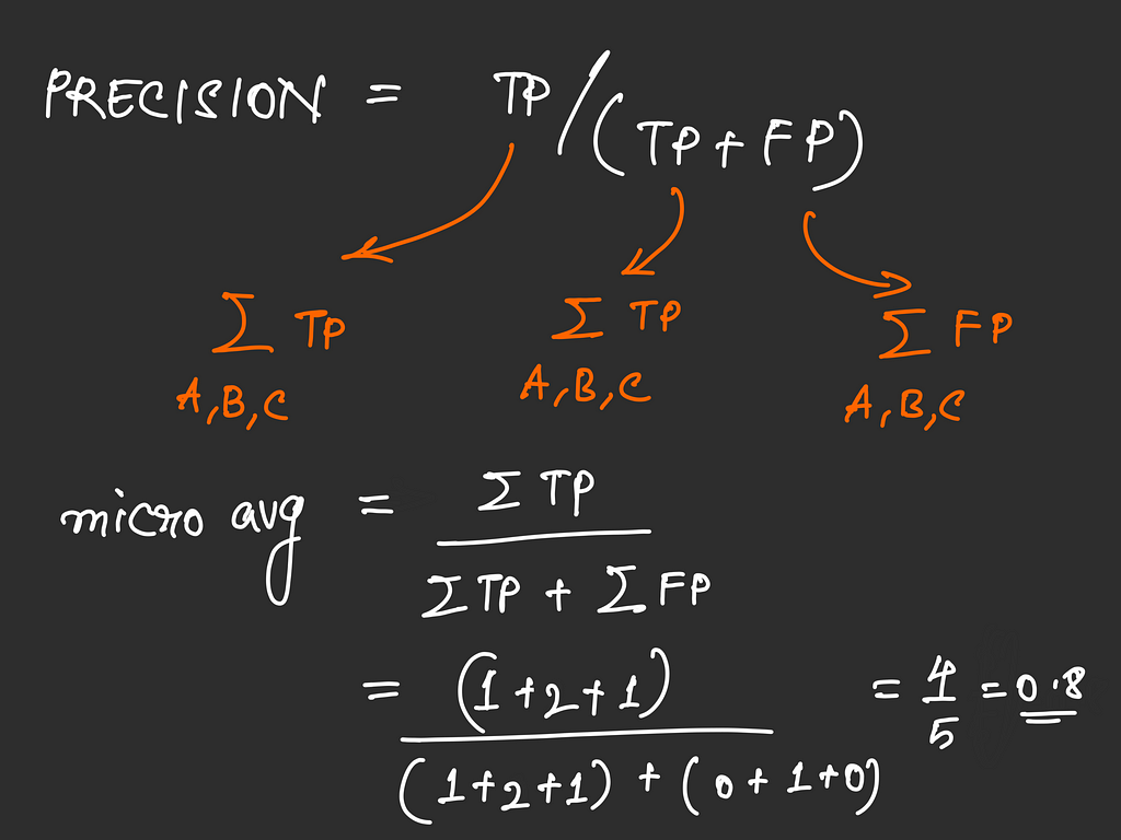
Micro average
The micro-average of a metric is calculated by considering all the TP, TN, FP and FN for each class, adding them up and then using those to compute the metric’s micro-average
For example, micro-precision would be:
micro avg (precision) = sum(Tp) / (sum(TP) + sum(FP))
For our example, we end up getting:
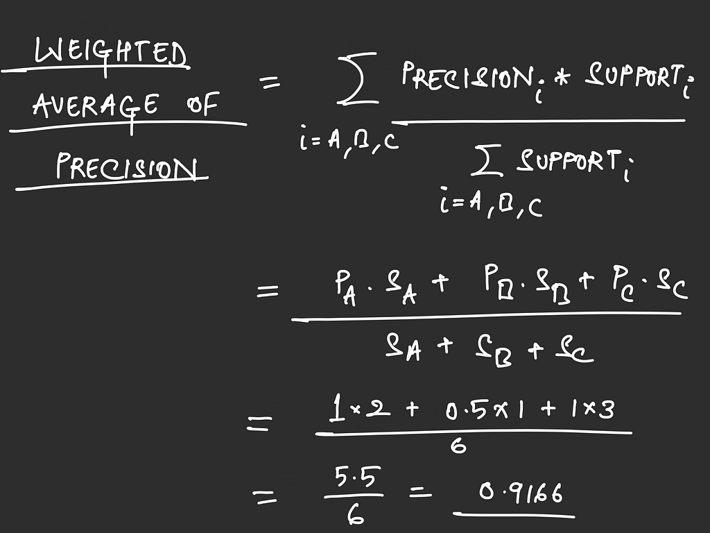
Weighted average
This is simply the average of the metric values for individual classes weighted by the support of that class.
Samples average
Here, we compute metrics for each sample and then average them. In our example, we have three samples.
expected   predicted
A, C        A, B
C           C
A, B, C     B, C
For sample #1, A and B were predicted, but the expected classes were A and C
So the precision for this sample would be 1 / 2, since out of the two predicted labels, only one was correct.
For sample #2, C was predicted, and C was expected.
So precision would be 1 for this sample — all predicted labels were expected.
For sample #3, B and C were predicted, but all three labels were expected.
Since all predicted labels were expected, precision would be 1. Note that though A wasn’t predicted, the missing label won’t hurt precision, it’ll hurt recall.
Averaging this, we get our samples average for precision.
(1/2 + 1 + 1) / 3 = 5/6 = 0.833
These aggregates can be computed for recall and f1-score as well.
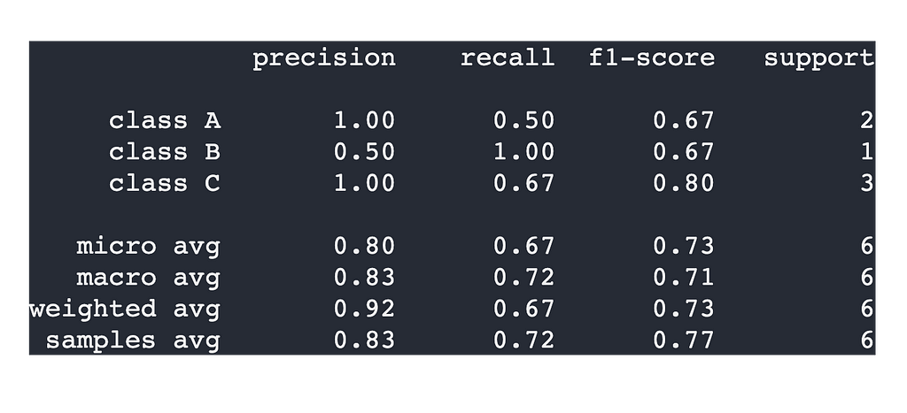
The Classification Report
Putting all this together, we end up with our classification report. Our computed values match those generated by sklearn. We’ll use sklearn’s metrics.classifiction_report function.
classification_report(
    y_expected,
    y_pred,
    output_dict=False,
    target_names=['class A', 'class B', 'class C']
)
Some common scenarios
These are some scenarios that are likely to occur when evaluating multi-label classifiers.
Having duplicates in your test data
Real-world test data can have duplicates. If you don’t remove them, how would they affect the performance of your model? The aggregate metrics generally used when evaluating classification models are forms of average. So the effect of duplicates comes down to whether these duplicated data points are correctly classified or not.
Your model predicts only some of the expected labels
When your model doesn’t predict every expected label but also doesn’t predict extra labels, you’ll see higher precision values along with lower recall values.
Whatever your model predicts, it's doing it correctly (high precision) but it's not always predicting what’s expected (low recall).
Your model predicts more labels than are expected
This is the opposite of the previous scenario. Since your model is predicting extra labels, those extra classes would end up with lower precision (since those predictions aren’t expected). At the same time, your model is predicting all the expected labels too, so you’d end up with high recall scores.
High precision — High recall
This is the ideal scenario, where both precision and recall are high. Intuitively, this means that when our model predicts a particular label, that’s most often an expected label, and when a particular label is expected, our model generally gets it right.
High Precision — Low Recall
This means that our model is really selective in its predictions. When a data point is particularly difficult to label, our model chooses to not take the risk of predicting an incorrect label. This means that when our model predicts a particular label, it is more often than not correct (high precision), but the same isn’t true the other way around (low recall).
Low Precision — High Recall
In this case, our model is pretty lenient in its predictions. It is more likely to assign a label to a data point even if it’s not completely sure. And because of this, our model is likely to assign incorrect labels to certain data points, leading to a drop in precision.
Thresholding to improve results
Most algorithms use a threshold of 0.5. This means that predictions with confidence greater than 0.5 are considered to belong to the positive class, while less confident predictions aren’t considered.
How does this relate to the entire precision-recall discussion? Well, think about what would happen if you modified this threshold.
If you increase your threshold, you’re getting more stringent about what your model predicts. Now that only predictions with high confidence are assigned, your model is more likely to be right when it predicts a class, leading to high precision. At the same time, your model may miss expected labels that had low confidence, leading to a lower recall.
On the other hand, reducing your model’s classification threshold would mean that your model is lenient about its predictions. That would mean that your model is more likely to predict expected labels though they may have been low-confidence decisions, meaning that you’ll have a high recall. But now that your model is less strict, it’s likely that the labels it assigns aren’t part of the expected labels, leading to lower precision.
Balancing recall and precision
As we just saw, there’s a tradeoff between precision and recall. If you make your model highly selective, you end up with better precision, but risk facing a drop in recall, and vice versa.
Between these two metrics, what’s more important depends on the problem you’re trying to solve.
Medical diagnostic tools, like skin cancer detection systems, can’t afford to label a cancerous case as a non-cancerous one. Here, you would want to minimize the false negatives. This means that you’re trying to maximize recall.
Likewise, if you consider a recommendation system, you’re more concerned with recommending something that customers may not be interested in than with not recommending something they would be interested in. Here, fall negatives aren’t an issue — the goal is to make the content as relevant as possible. Since we’re reducing false positives here, we’re focusing on precision, rather than recall.
Note #1: Keep forgetting the difference between precision and recall?
A good way to remember the difference between what precision and recall represent is explained in this answer by Jennifer on the data science StackExchange site:
When is precision more important over recall?
Note #2: Are there other metrics than the ones discussed in this post?
Definitely. Different kinds of problems have different metrics that work best for that particular case. Even for the case we just discussed — multi-label classification — there’s another metric called a Hamming Score, which evaluates how close your model’s predictions are to what’s expected. You can think of it as a more forgiving kind of accuracy for multilabel classifiers.
A good starting point would be this excellent TowardsDataScience article by Rahul Agarwal.
The 5 Classification Evaluation metrics every Data Scientist must know
Conclusion
Evaluating your model using the right metrics is imperative. Realizing halfway through your experiments that you were measuring the wrong thing is not a fun position to be in.
You can avoid this by finding out which metrics are the most relevant to your use case, and then actually understanding how these are computed and what they mean.
Hopefully, this article gave you an idea of how multi-label classifiers are evaluated. Thanks for reading!
Evaluating Multi-label Classifiers was originally published in Towards Data Science on Medium, where people are continuing the conversation by highlighting and responding to this story.
from Towards Data Science - Medium https://ift.tt/3GGJ633
via RiYo Analytics


No comments