https://ift.tt/31BtoGr Exploring basic NLP preprocessing and Encoder-Decoder architecture ubiquitous in all Seq2Seq tasks Image via Adobe...
Exploring basic NLP preprocessing and Encoder-Decoder architecture ubiquitous in all Seq2Seq tasks

Machine Translation is undoubtedly one of the most worked upon problems in Natural Language Processing since the inception of research in the domain. Through this tutorial, we shall explore an Encoder-Decoder NMT model employing LSTM. For simplicity, I resort to discussing better performant architectures based on Attention mechanisms for a later post.
Dataset
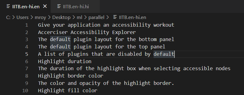
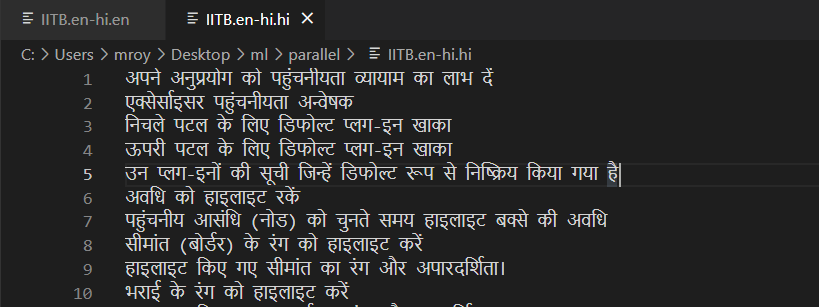
I have used the IIT Bombay English-Hindi Corpus as the dataset for the tutorial as it is one of the most extensive corpora available for performing English-Hindi translation task. The data present is essentially a list of sentences in two separate files for each language that looks as:
Preprocessing
As basic preprocessing, we need to remove punctuation, numerals, extra spaces and convert them to lowercase. Pretty standard stuff encapsulated within a function:
One important thing to note is the notoriety of the Hindi sentences present. In addition to running the sentences through the above function, they need to be sanitized to remove the english characters they contain as well. This actually caused NaN bugs during training which consumed a lot of time in debugging. We can avert the issue by replacing any english character with empty string using regex, as shown below:
hindi_sentences = [re.sub(r'[a-zA-Z]','',hi) for hi in hindi_sentences
LSTMs generally don’t tend to perform for very long sequences (although better than RNNs but still no way comparable to Transformers). Hence, we reduce our dataset to contain sentences not exceeding in length by 20 words. Also for demonstration purpose, we consider a total of 50000 sentences to keep training time low. We can achieve the following as:
Preparing the Data
During translation, how will our model know when to begin and end? We use <START> and <END> tokens specifically for this purpose, which we prepend and append to our target language. This can be achieved as a one-liner as shown:
hi_data = ['<START> ' + hi + ' <END>’ for hi in hi_data]
Although the exact usage of this voodoo step might not be clear at the moment but it is quite easy to understand once we discuss the architecture and how things exactly work. At this point, we still have our data in the form of character sentences, which needs to be transformed into numeric representations for the model to work upon. In specific, we need to create a word-index representation for both the English and Hindi sentences. We can use tensorflow’s inbuilt tokenizer to relieve ourselves of manually performing this as shown:
One important parameter to note here is oov_token, which essentially stands for Out-of-Vocabulary. This is specially used in the case we want to restrict our vocabulary to say have only top 5000 words. In that case, any unpopular word (rank of word based on instance count > 5000) would be replaced by the parameter value and treated as not contained in vocabulary. This way we can relax our model to disregard any influence caused by obscure and rare words present in the dataset. Another crucial point to note is that we add 1 to the vocab size for both English and Hindi words to accomodate for padding digits (discussed later).
Prepare Decoder Inputs and Outputs
The way the NMT model works can be understood as a two phase process. During the first phase, the encoder block ingests the input sequence one word at a time. Since, we are using an LSTM layer, with the consumption of each word, the internal state vectors [h, c] will get updated. After the final word, we care only about the final values of these vectors to be fed into the decoder. The second phase then works by ingesting the encoder’s final [h,c] vector and also consuming each token of the target sentence, beginning with <START>. The output produced for each token will be matched with what is expected and error gradients are generated to update the model. Upon exhaustion of the target inputs, we expect our model to produce an <END> token denoting the completion of this data-sample. This can be better understood from the following diagram.
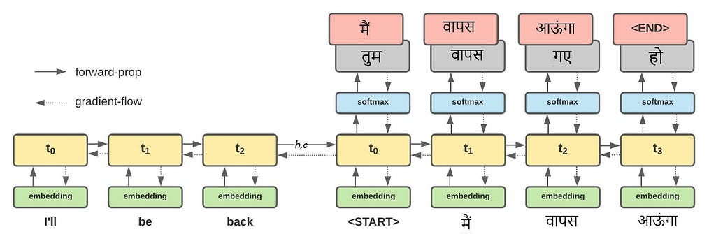
We demonstrate the translation of Arnold’s famous dialogue from The Terminator (1984) ~ “I’ll be back”. As, we can see the decoder LSTM is initialized with the final [h,c] of the encoder. We can understand this step as a transfer of thought/summary of the input sentence to the decoder LSTM. The grey boxes indicate the output of the LSTM unit and the red boxes the target token at each time-step. When the first token <START> is fed into the decoder LSTM, we expect it to produce मैं, however it produces तुम accounting for a contribution to the error gradient (to be used for backpropagation through time). From the above diagram, it is clear that we ought to realign our target sentence in the following manner, which can be achieved using the code block below:
decoder-input:  <START> मैं   वापस  आऊंगा
decoder-output:   मैं   वापस आऊंगा <END>
Note: LSTMs work only with fix-length sequences, hence we need to perform padding.
Model Architecture
To keep training time low yet have sufficient dimensionality to capture the variance in data, we choose to have our vector dimensionality (d_model) to be 256.
As demonstrated by the above snippet, we care about the final internal state [h, c], and not the output of the encoder LSTM.
As described above, the decoder LSTM is initialized by the encoder internal states and its output is fed into a Dense layer with number of units equal to the target vocab size (hindi_vocab_size) with a softmax activation. The idea is to generate a probability distribution over all the words of the target vocabulary. Choosing the one with highest value means that this particular token is the highest probable, which is exactly what we do here. We use SparseCategoricalCrossEntropy as the loss function to be optimized.
Training and Results
I trained the above network for around 10 epochs on a training-test-split of 95%-5%. Considering the limited power and disconnection in google colab (if kept in idle training), I had to compromise on a fairly underwhelming model and limited training data, with which I achieved a training and validation accuracy of ~ 45% at the moment 😢. I hope to improve the score and update the post accordingly with any changes I make in the code.
Making Inference
The inference model reuses the trained encoder and decoder models. The encoder portion takes in the trained embedding layer as input and outputs the final [h, c] (essentially pulling in the LSTM layer as well), to be used by the decoder. The decoder in a similar fashion takes as input the trained target embedding layer and the encoder final states [h, c] for the first token. For each subsequent token, we provide the previous decoder internal states (to essentially give the context of current word and predict the next on the basis of that). This is better understood from the inference algorithm below:
During the translation step, we feed the english sentence into the encoder and get the output states [h,c]. The main translation happens in lines (10–18), where we get the next word for the current word and update the internal state to be used for the next step. This cycle is repeated until we get an <END> token or reach maxlen tokens.
English to Hindi Neural Machine Translation was originally published in Towards Data Science on Medium, where people are continuing the conversation by highlighting and responding to this story.
from Towards Data Science - Medium https://ift.tt/3BM9jtf
via RiYo Analytics


No comments