https://ift.tt/3xwwd7n What is NLP? How do we perform NLP? Just started with the SpaCy package? Here is a complete guide on performing NLP ...
What is NLP? How do we perform NLP? Just started with the SpaCy package? Here is a complete guide on performing NLP and its associated concepts.

COVID-19 has affected the lives of many through losing beloved ones, being laid-off from jobs, and social distancing from the world. However, during the digital era, people did not stop sharing their thoughts, comments, or feelings with the world — they did it through the power of social media.
In this article, we will go through the main concepts of NLP project, including the data selection, exploratory data analysis, NLP preprocessing, NLP models (statistical/neural language models), and metrics selection. The dataset of interest is the COVID-19 tweet dataset on Kaggle, while all NLP-related tasks are performed using SpaCy.
The Setup
In this article, I used the Coronavirus Tweets NLP to create a model that classifies sentiments of tweets simply by observing the content of the tweets. I show working code using spaCy and then evaluated through models using simply naive Bayes, logistic regression, support vector machine, to neural networks, such as BERT.
The environment I used was Python 3.7 on a venv virtual machine based on a Deepnote notebook. The packages involved are:
- spaCy: a fast, production-level NLP library.
- matplotlib.pyplot: a common package for data visualization in Python
- scikit-learn: a simple and useful package for data analysis and machine learning.
- pandas: a common, flexible, and easy-to-use data analysis and manipulation tool on Python.
These packages were the foundation of the preprocessing, training, and visualization throughout the analysis.
The Data
The data I used is the Coronavirus Tweets NLP dataset on Kaggle. The data was collected via Twitter and went through manual tagging, resulting in 41,157 samples on the training data and 3,798 samples in the validation data. It consists of 4 columns as the following:
- Location: Location of the publication of the tweet
- Tweet at: Time of the publication of the tweet
- Original Tweet: Text of the tweet
- Label: Human-labeled sentiment, ranging from extremely negative to extremely positive.
There were also two additional columns, UserName and ScreenName, which were discarded for privacy reasons.
Exploratory Data Analysis
Before training the model, I did some exploratory data analysis (EDA) on the data, mainly through Pandas Profiling, a powerful package that creates a user-friendly interface for EDA of any datasets (see below). Based on the report, I also conducted some manual EDA visualizations to present a more specific analysis on the data.
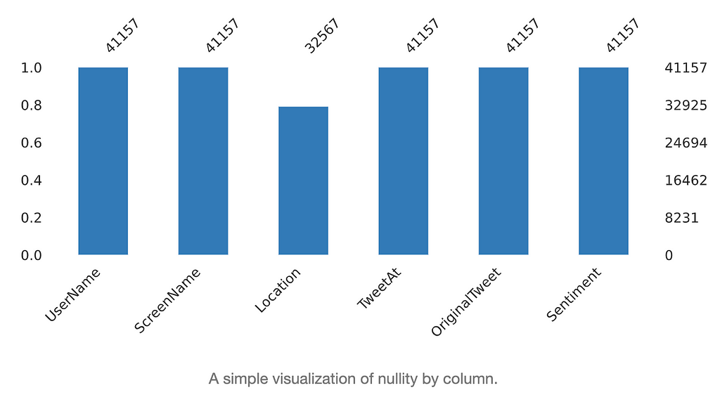
- Missing data (NAs)
Figures to the left show the missing data in the dataset. We observed that missing data is only present at the location column.
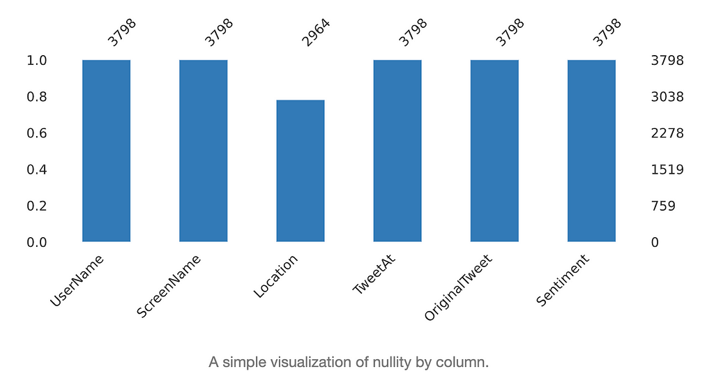
We also see that the percentage of missing data in the location columns is similar between the training set and test set, both at around 30%.
After further inspection of the location columns, we find that the data contains inconsistency in the labeling of location names and longitude and latitude data, making the data less usable on top of missing data.
- Balance of Categories
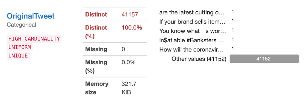
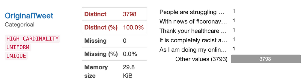
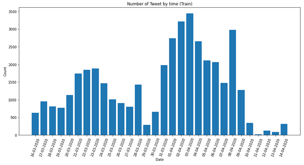
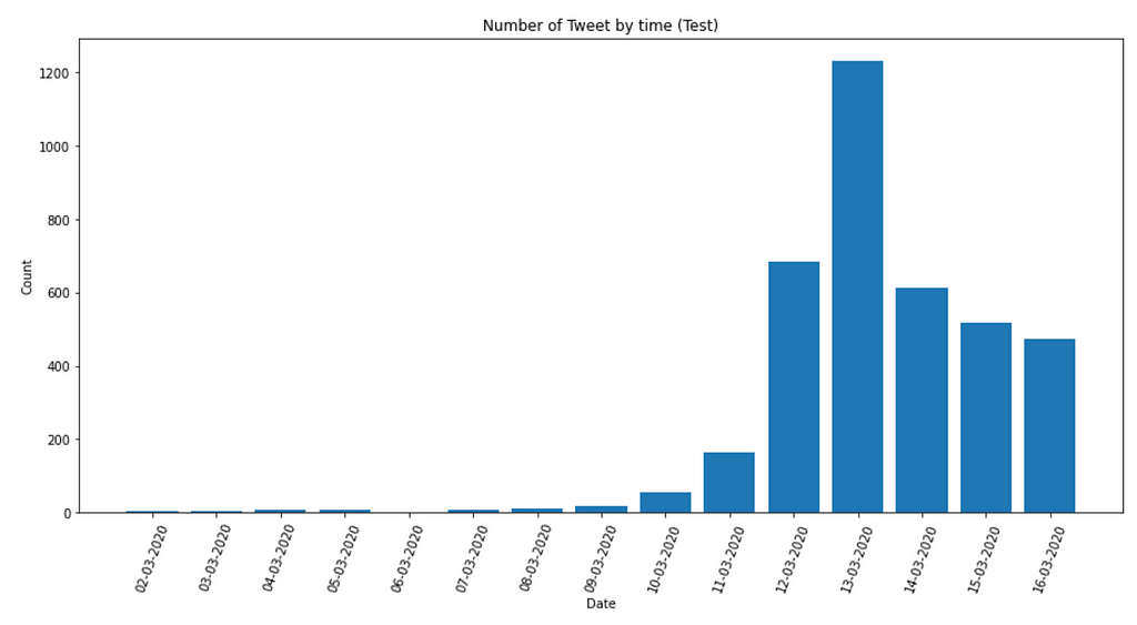
To further explore the data, I looked at the distribution of the different columns using Pandas Profiling. The OriginalTweet column is completely unique. While the TweetAt column has a distribution that is clearly divided by dates, which, though highly unlikely, could confound the sentiment classification between the Sentiment and OriginalTweet columns. Therefore, I decided to resplit the data during the preprocess section.
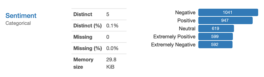
On the other hand, the Sentiment column shows categories that are less balanced, with positive having the most data and extremely negative having the least. However, this is not true for the test set, which has more negative than positive tweets shown below. Hence, I invested more into this in order to determine if this would be another confounder to the analysis.
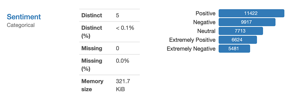
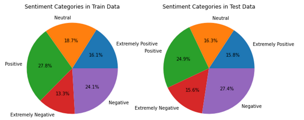
To make it easier to compare, I build pie charts for each of them and found that the differences in the percentage are not significant as the Pandas Profiling report initially shows, with all categories only changing within 3%. Nevertheless, due to the time dependencies of the TweetAt column, I had to reshuffle the whole dataset.
For more exploratory analysis on the data, please check out the reports generated using Pandas Profiling by implementing the code on a local Jupyter Notebook.
Preprocessing
After understanding the raw data, I combined the train and test data and took half of the data to perform two splits, each splitting 20% of the original data, creating three datasets (sampling 50% of the data was due to computational limitations when training the models):
- Train set: 80% of all data, used for training.
- Test set:16% of all data, used for testing the training.
- Validation set: 4% of all data, used for testing the models on unseen data.
This was done through the following code:
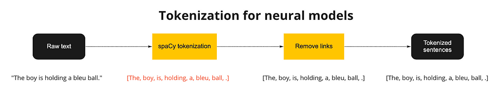
The next step is to complete a series of natural language processing (NLP) procedures in order to “clean” the tweets into the tokens, which could be digested by the different models. We can use the analogy of “cooking” to describe this process.
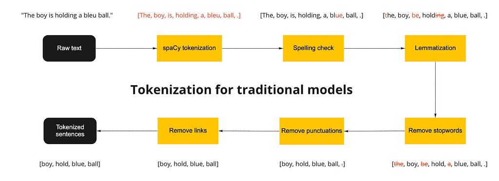
The original tweets are the raw ingredients, such as carrots. To bake a carrot cake, we would first need to wash the carrot to remove unwanted dirt. In NLP, we need to first remove unwanted characters, such as urls, emojis, hashtags, etc. This depends on the task at hand. For example, hashtags could be important if you want to find the association between hashtags and the text.
In my case, I did not want any of these, so I remove all of these via the methods including:
- Remove punctuations from the string library
- Remove stopwords (function words, e.g., to, in, etc.) using spaCy
- Remove URLs using regular expression (from re package)
Next on, if the carrot has some mold or unwanted parts on it, it is natural to cut that small part off or wash it again. This is similar to the spelling correction part of the preprocessing, where we use fuzzy matching to adjust some misspellings back to their original form. Specifically, Levenshtein distance (i.e., edit distance) was used to calculate the number of differences between the written word and its possible corrected form. I used spellCheck package for this task since it can be directly added to the spaCy pipeline and the edit distance can be set manually.
After that, we do not need the skin of the carrot, though it does have some values and benefits when attached to the carrot. This is similar to the lemmatization process where we remove meaningful semantic sections of the row to reduce the words into their core form. For example, the word “running” has a double n and -ing suffix. When using it in reality, we would only want the stem word “run”. However, when you want to identify the time aspect (or tense) when doing part-of-speech tagging (POS), this suffix -ing becomes substantial as it tells us that the sentence is in a progressive tense.
Finally, we diced up the carrots into chunks for cooking later on. This is the process of tokenization, where we separate the words with their stem words for later manipulation with different models. In this case, we used the nlp function in spaCy, which automatically finished the tokenization process by identifying the spaces in between words. We can also call the whole preprocess a tokenization process as we are ultimately inputting the sentences and outputting the core tokens of each sentence.
Now, we have the sentences tokenized, but the labels are still under the string format. Since the labels are comprised of “Extremely Negative”, “Negative”, “Neutral”, “Positive”, and “Extremely Positive”, we can label each class from 1 to 5
The Models
After preparing all the tokenized sentences, we now can use train the models using are preprocessed data. The models I chose can be separated into two categories. The first one is statistical language models, including Naive Bayes, logistic regression, and support vector machines (SVM), and the second one is neural language models, including CNN and BERT models.
Statistical Language Models
Statistical language models use a probabilistic approach to determine the next word or the label of the corpus. Common probabilistic models use order-specific N-grams and orderless Bag-of-Words models (BoW) to transform the data before inputting the data into the predictor. For example, we are performing a classification task in this article; therefore, the bag-of-words model, essentially the frequency table of all tokens, was performed on the corpus via scikit-learn’s CountVectorize before inputting in probabilistic models below.
To perform the preprocessing of any data mentioned in the last section, the bag-of-words vectorization, and the classification from multiple models, I used scikit-learn’s Pipeline module that groups the cleaning of data, the vectorization, and the classification into one pipeline — that allows simpler data processing step for the transfer learning of the algorithm with other data and models.
- Naive Bayes (NB)
Naive Bayes (NB) is a common model for document classification. The main concept of Naive Bayes is to use the Bayes’ Theorem to estimate the joint probability of all the different words conditioned on each label you have.
In other words, imagine you have two brands of chips, each with its unique shape, color, and flavor. By identifying the common trends in the shape, color, and flavor of each individual chip, we can guess the brand of an unknown chip simply through its characteristics. Here, we can relate this concept to the formal concepts of Naive Bayes through the following:
- The brands of chips are the labels
- The characteristics of individual chips are the frequencies of each token
- Bayes’ Theorem can correspond to the common trends in each brand
In reality, we simply use scikit-learn’s MultinomialNB function to conduct Naive Bayes after transforming the data to a bag-of-words model:
For a more complete explanation of Naive Bayes, please read this article from Gustavo Chávez.
- Logistic Regression
Although most common in binary classification problems, multinomial logistic regressions are an alternative to Naive Bayes for multi-class problems. The main concept of logistic regression is to use linear combinations of the observed features to estimate the particular value and the corresponding label.
Going back to the chip example, for each brand, we assign values to the shape, color, and size of each chip and add them up to a certain value. If the value is higher than a threshold, we would view the chip as one brand, and if it is lower than, then it would be the other band. This is the general logic of a binary logistic regression, where the linear combination of observed features refers to the adding of the different assigned values for the characteristics of the chips.
Here, we used use scikit-learn’s LogisticRegression function to conduct multinomial logistic regression after transforming the data to a bag-of-words model:
If you wish to learn more, please refer to this wiki page on multinomial logistic regression.
- Support Vector Machine (SVM)
Support vector machine (SVM) is also a common model for classification. The advantage of SVM is that it generates a hyperplane decision boundary, meaning that non-linear characteristics can be used for classification as well.
Using the chip example, we can imagine we throw a bunch of chips from the two brands on a table. We then order each chip by its color on one axis and its size on the other axis. We would be able to know which chip belongs to which brand at this time. However, the chips sometimes are mixed and, hence, we cannot draw a straight line to separate the two brands of chips. Now, we find a way to project these chip into the 3D projection on the table, where each chip are also separated by the spiciness of the chip. By doing so, we can put a paper in the 3D projection that perfectly separates the two brands. Finally, we project the paper onto the table, where a squiggly line perfectly separates the two brands.
Although much more complicated, this is the simplistic explanation of using SVM algorithm (the 3D projection transformation) to find the non-linear decision boundary (the paper).
Similar to before, we used use scikit-learn’s SVC function to conduct SVM after transforming the data to a bag-of-words model:
For more information, please watch this YouTube series by StatQuest.
Neural Language Models
Neural language models utilize the current advances in neural networks, which generalized the models better than past statistical models. Although each neural network uses a fairly different structure to optimize the classification, in NLP, word embeddings are considered the breakthrough technology that enables substantial growth in the past couple of years.
Word embeddings are vectorized representations of the words that mark words that are similar closer together mathematically. This can be one-hot encoded tokens trained by yourself, but also pre-trained embeddings from big tech companies or academic institutions, such as Word2Vec and BERT embeddings by Google, or GloVe from Stanford.
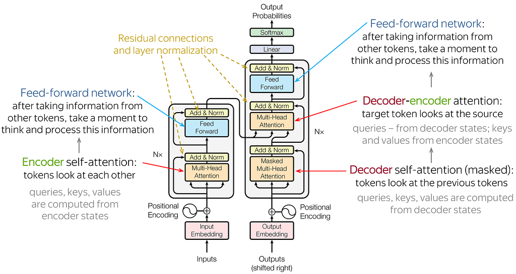
In addition to word embeddings, the architectures of the models can influence the accuracy of the model even with the same data. One of the most advanced architectures in NLP currently is Transformers. The transformer architecture takes inputs from a sequence and outputs a sequence. In between, the sequence will first go through an encoder stack and then go through a decoder stack, which both are equipped with attention mechanisms (e.g., self-attentions). Although this sounds really technical, we can think of encoder-decoder as morse code where we encode English text into long and short signals before outputting through a decoder that translates back into English.
Attentions, on the other hand, are enables the model to focus on other words in the input that is closely related to that word. Think of it as visual attention — where our eyes focus on specific parts of a picture based on what we’ve seen before. For example, look at the picture below. When looking at her sunglasses, we naturally focus on her noise due to the close proximity. You might think the distance between the parts is all that matters but if you look at the right side of her hair, we also pay our attention to the left side as they are both parts of “her hair” even though her face is in between. Despite not being a precise analogy, attention in transformers works in a similar way

Take the following sentence as an example, when we focus our attention on the word “ball”, its association with the adjective “blue” and the verb “holding” would be stronger than the subject “boy” since “ball” is more likely to be “hold” regardless of it being held by a “boy”, a “girl” or any other person.

Attention formalizes this context-driven information mathematically and accounts for this association when computing the outcome, which is usually better than statistical bags-of-word models as “context” information can not be stored.
For more information, please check out this series by Ketan Doshi or this article by Lena Voita.
SpaCy’s textcat ensemble
For my first implementation, I chose spaCy’s internal textcat ensemble model, which combines a Tok2Vec model with a linear bag-of-words model using the transformer architecture. To execute this on spaCy, we need to first understand how spaCy trains models.
- Configuration systems
Due to the complexity of the settings and hyperparameters that could be inputted for each layer in a neural network. Configuration system in spaCy allows the developer to store and write these parameters in a clean way and to minimize redundant work if a parameter is global. Rather than creating a long class for each individual layer of the neural network, we list out what we need in a .cfg file that can be called via command-line operations. We can quickly create one of these using SpaCy’s quickstart function in its documentation.
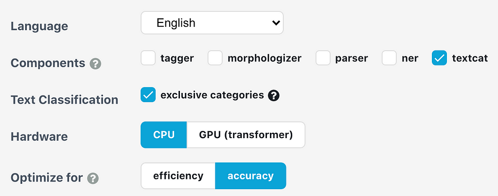
The specific choices I made are documented in the image above. This outputs a .cfg file that is called base_config.cfg, which would be used to fill in the actual config.cfg using the command-line prompt below.
Before training the model, we also need to process the data differently as the input now is not a bag-of-word model but rather raw text. This was done through three steps:
The first step is to remove unwanted text, such as removing URLs from the raw text. In this case, removing stopwords and punctuations is not necessary as spaCy’s transformer model connects with a tokenizer automatically. Also, lemmatization is not necessary as prefixes and suffixes contain valuable context to the word, which is helpful for attention in determining associations.
The second step is to conduct one-hot encoding on the categories, transforming the categories into a dictionary of [0,1] corresponding to the actual label of the text. For example, a “Positive” label would be {"Extremely Positive": 0, "Positive": 1, …,"Extremely Negative": 0}.
The third step is to convert the output of these data into binary files called .spacy in order to execute the training process in spaCy.
Finally, we can train these files using a command-line prompt in which we also specify the train data input, test data input, and model outputs.
Bidirectional Encoder Representations from Transformers (BERT)
Using the same configuration system, I retrained the data using a pre-trained BERT model on top of a RoBERTa-based pipeline called en_core_web_trf. The only that I changed was loading the spaCy’s pipeline and docs using en_core_web_trf rather than en_core_web_sm, which is the small standard English pipeline.
RoBERTa is an optimized version of BERT published in 2019 by Facebook. It improves on the BERT architecture, which is considered one of the state-of-the-art models for NLP text classification tasks. The main idea behind BERT is to use the encoder part of a transformer and conduct masked-language modeling, which means removing tokens in sentences and predicting them, as well as next sentence prediction, which is predicting the next sentence based on previous and later sentences.
We can think of masked-language modeling as filling in the gap of a sentence where the model is trained on filling the correct word for these sentences similar to the example below. 15% of the data was masked during the pre-trained BERT model.
FILL-IN THE GAP: The boy is __ a blue ball.
The next sentence prediction on the other hand is the large-scale version of masked-language modeling where the model masks complete sentences and uses the sentences before and after to predict the content. The weights for each layer in the encoder are then frozen after being trained on massive data to store the context between words and sentences.
This pre-trained BERT model is useful for transfer learning as the weights at each layer of the encoder will be predetermined. By doing so, we can add an additional layer to train the classification tasks based on the outputs of the pre-trained weights (usually consisting of contextual information of the sentences).
Going back to the cooking example, we can imagine that the chefs before already finished seasoning, cooking, and gathering all the necessary ingredients. Now, we only need to plate the food and decorate the dish with features that the customer wants. In this example, everything that happens before the plating is executed by the researchers that constructed the pre-trained model. What we only need to do is fine-tune the dish for our specific tasks (customers).
For more information on the BERT model, please check out this article.
The training process follows the same procedures as the previous model except that we need to create the .spacy files with the RoBERTa pipeline.
Then, we train using the same method as the previous model
The Result
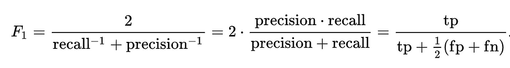
The main metric I used was the F1 score. This metric combines recall and precision using the following equation:
To understand what the F1 score means, we need to understand what precision and recall are.
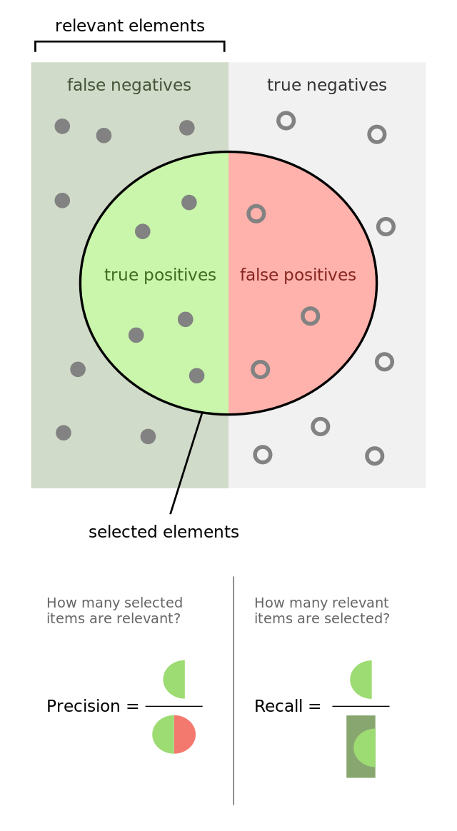
- Precision: Of all the predicted positive values, how many are actually positive? This metric shows the accuracy of the model when we only look at the positive cases.
- Recall: Of all the actually positive values, how many are predicted to be positive? This metric shows how well the model performs on detecting the actual positive values.
For any given model, the usual goal is to maximize both precision and recall, however, there is often a trade-off between the precision and recall metrics. To get a general understanding of both aspects of the accuracy of the model, F1 score is calculated as the harmonic average between the two metrics. This is used as simply averaging the two values would decrease the importance of each individual value.
Model result
The result of each model is shown below:
- Statistical Language Models Result
Naive Bayes model
Logistic Regression model
SVM model
From the three models, we see that the accuracy of the logistic regression and SVM are both around 0.55 while the naive Bayes model has the worst accuracy at around 0.45.
- Neural Language Models Result
SpaCy’s standard model
The textcat ensemble model by spaCy converged at an accuracy of 0.63.
BERT
The fine-tuned pre-trained BERT model converged at an accuracy of 0.61.
Comparison
From these results, we see that neural networks improve the F1 accuracy results. However, the training time of the models took a really long time on a CPU machine (12 hours for 10 epochs) even with pre-trained BERT (6 hours for 10 epochs) compared to the statistical models (~2.5 hours per model). This is because although neural models usually have a better accuracy than the traditional models, the training of neural models requries a large computation power. Therefore, without a sufficient CPU or GPU or with a large dataset, the training of neural models could take days. Hence, the trade-off between the computation time and the accuracy is something that needs to be taken into consideration before running a specific task.
Example of individual tweets
To check out the neural language model prediction of individual tweets, I tested out an example from the validation set. The following are an example of one tweet for both neural language models.
This is the standard spaCy model:
It shows a negative categorization in both the predicted and original text, with a 0.80 probability of it being negative (truncated).
For the pre-trained BERT model, the results show a 0.94 probability of it being negative.
Although these results sound encouraging, the model accuracy is still limited on the data it was trained on. Therefore, due to the human-labeling process for this dataset, there could be errors by humans and propagate through the model during training. This would appear mostly during the prediction of tweets outside the current dataset, which is inevitable but could be mitigated by introducing the model to other data. This would be preferable to reduce the data dependency of the model and increase the robustness for general purposes.
The Summary
In this article, we work through the end-to-end process of building a text classification model using spaCy and COVID-19 tweet datasets. We went through the process of the exploratory data analysis and preprocessed the data accordingly. We then trained statistical models and neural models to observe their advantages and disadvantages. In the end, we evaluated the models based on the F1 accuracy metrics for each model.
In addition, we found out that neural networks generally have a better performance than statistical models; however, the training time for the neural network is significantly longer if no GPUs are installed. Hopefully, this article can help you understand what NLP text classification is and how to produce a model using spaCy!
The References
Code Reference
Data Source from Kaggle
- A. Miglani, Coronavirus Tweets NLP (2020), Kaggle
Articles & Videos
- Standford NLP, Tokenization (2008), Cambridge University Press
- J. Brownlee, Gentle Introduction to Statistical Language Modeling and Neural Language Models (2019), on Deep Learning for Natural Language Processing in Machine Learning Mastery
- J. Brownlee, What Are Word Embeddings for Text? (2017), on Deep Learning for Natural Language Processing in Machine Learning Mastery
- K. Doshi, Transformers Explained Series (2020), on Towards Data Science
- D. Subramanian, Building a Sentiment Classifier using spaCy 3.0 Transformers (2021), on Towards Data Science
- SpaCy, SpaCy 3.1 documentation (2021)
Complete Guide to Perform Classification of Tweets with SpaCy was originally published in Towards Data Science on Medium, where people are continuing the conversation by highlighting and responding to this story.
from Towards Data Science - Medium https://ift.tt/3lfw57o
via RiYo Analytics


ليست هناك تعليقات