CNN-LSTM based Models for Multiple Parallel Input and Multi-Step Forecast

https://ift.tt/3HyKVzg CNN-LSTM-Based Models for Multiple Parallel Input and Multi-Step Forecast Different neural network approaches for m...

https://ift.tt/3HyKVzg

CNN-LSTM-Based Models for Multiple Parallel Input and Multi-Step Forecast

Different neural network approaches for multiple time series and multi-step forecasting use cases, and real-life practices of multi-step forecasting

Time series forecasting is a very popular field of machine learning. The reason behind this is the widespread usage of time series in daily life in almost every domain. Going into details for time series forecasting, we encounter lots of different kinds of sub-fields and approaches. In this writing, I will focus on a specific subdomain that is performing multi-step forecasts by receiving multiple parallel time series, and also mention basic key points that should be taken into consideration in time series forecasting. Note that forecasting models differ from predictive models at various points.

Photo by Faruk Kaymak on Unsplash

- Problem Definition

Let's think about lots of network devices spread over a large geography, and traffic flows through these devices continuously. Another example might be about lots of different temperature devices which measure the temperature of the weather in different locations continuously or another one might be to calculate the energy consumption of numerous devices in a system. We can just extend these kinds of examples easily. The goal is simple; forecast the next multiple time steps; this corresponds to forecasting traffic value, temperature, or the energy consumption of many devices respectively in our case.

The first thing that comes to mind is certainly modeling each device separately. I think we will probably get the highest forecast results. What about if there are more than 100 different devices or even more? That means designing 100 different models. It is not much applicable considering the deploying, monitoring, and maintenance costs. Therefore, we aim to cover the entire problem with just a single model. I think it is still a very popular and searching field of time series forecasting, although time series forecasting has been on the table for a long time. I encounter lots of different academic research in this field.

This problem might also be defined as seq2seq prediction. In particular, it is a very common case in speech recognition and translations. LSTM is very convenient for these kinds of problems. CNN can also be considered as another type of neural network and is commonly used in image processing tasks. Typically, it is used in feature extraction and time series forecasting as well. I will mention the appliance of LSTM and CNN for time series forecasting in multiple parallel inputs and multi-step forecasting cases. Explanation of LSTM and CNN is simply beyond the scope of the writing.

To make it more clear, I depict a simple data example below. It is an example of forecasting traffic values of 3 different devices for the next 2 hours by looking at the previous 3 hours time slots.

Image by Author — Figure 1

- Data set Description

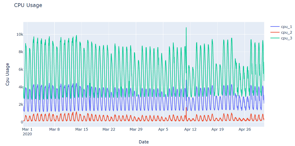
In this writing, I will utilize a data set consisting of a CPU usage of 288 different servers within 15 minutes time interval. For simplicity, I will narrow down the scope into 3 servers.

Data Set Example, Image by Author — Figure 2

- Pre-modeling Steps

Pre-modelling is very critical in neural network implementations. You mostly can not simply feed the neural network with raw data directly, a simple transformation is needed. However, we should apply a few more additional steps to the raw data before the transformation.

The following is for pivoting the raw data in our case.

df_cpu_pivot = pd.pivot_table(df, values=’CPUUSED’, 
 index=[‘DATETIME’], columns=[‘ID’])

The following is for interpolating the missing values in the data set. Imputing null values in time series is very crucial on its own, and a challenging task as well. We don’t have many null values in this data set and imputing null values is beyond the scope of this writing, therefore I perform a simple implementation.

for i in range(0, len(df_cpu_pivot.columns)):
 df_cpu_pivot.iloc[:,i].interpolate(inplace = True)

The first thing before passing into the modeling phase, at the very beginning of the data preprocessing step for time series forecasting is plotting the time series in my opinion. Let's see what tells the data to us. As I mentioned before, I select only 3 different servers for simplicity. As it can be seen, all of them follow very similar patterns in different scales.

import plotly
import plotly.express as px
import plotly.graph_objects as go

df_cpu_pivot.reset_index(inplace=True)
df_cpu_pivot['DATETIME'] = pd.to_datetime(df_cpu_pivot['DATETIME'])

trace1 = go.Scatter(
 x = df_cpu_pivot[‘DATETIME’],
 y = df_cpu_pivot[‘HSSFE-hssahlk01CPU-0’],
 mode = ‘lines’,
 name = ‘cpu_1’
)
trace2 = go.Scatter(
 x = df_cpu_pivot[‘DATETIME’],
 y = df_cpu_pivot[‘HSSFE-hssumrk03CPU-29’],
 mode = ‘lines’,
 name = ‘cpu_2’
)
trace3 = go.Scatter(
 x = df_cpu_pivot[‘DATETIME’],
 y = df_cpu_pivot[‘HSSFE-hssumrk03CPU-4’],
 mode = ‘lines’,
 name = ‘cpu_3’
)

layout = go.Layout(
 title = “CPU Usage”,
 xaxis = {‘title’ : “Date”},
 yaxis = {‘title’ : “Cpu Usage”}
)
fig = go.Figure(data=[trace1, trace2, trace3], layout=layout)
fig.show()

Cpu usage — Figure 3

The next step is to split the data set into train and test sets. It is a bit different in time series from conventional machine learning implementations. We can intuitively determine a split date for separating the data set.

from datetime import datetime
train_test_split = datetime.strptime(‘20.04.2020 00:00:00’, ‘%d.%m.%Y %H:%M:%S’)
df_train = df_cpu_pivot.loc[df_cpu_pivot[‘DATETIME’] < train_test_split]
df_test = df_cpu_pivot.loc[df_cpu_pivot[‘DATETIME’] >= train_test_split]

We also normalize the data before feeding it into any neural network model because of its sensitivity.

from sklearn.preprocessing import MinMaxScaler
cpu_list = [i for i in df_cpu_pivot.columns if i != ‘DATETIME’]
scaler = MinMaxScaler()
scaled_train = scaler.fit_transform(df_train[cpu_list])
scaled_test = scaler.transform(df_test[cpu_list])

And the final stage is to transform both train and test set into an acceptable format for neural networks. The following method can be implemented to transform the data. It simply expects 2 parameters except for the sequence itself, which are time lag(steps of looking back), and forecasting range respectively. You can also take a look at TimeSeriesGenerator class defined in Keras to transform the data set.

def split_sequence(sequence, look_back, forecast_horizon):
 X, y = list(), list()
 for i in range(len(sequence)): 
   lag_end = i + look_back
   forecast_end = lag_end + forecast_horizon
   if forecast_end > len(sequence):
     break
   seq_x, seq_y = sequence[i:lag_end], sequence[lag_end:forecast_end]
   X.append(seq_x)
   y.append(seq_y)
 return np.array(X), np.array(y)

An LSTM model expects data to have the shape; [samples, timesteps, features]. Similarly, CNN also expects 3D data as LSTMs.

# Take into consideration last 6 hours, and perform forecasting for next 1 hour
LOOK_BACK = 24
FORECAST_RANGE = 4
n_features = len(cpu_list)

X_train, y_train = split_sequence(scaled_train, look_back=LOOK_BACK, forecast_horizon=FORECAST_RANGE)
X_test, y_test = split_sequence(scaled_test, look_back=LOOK_BACK, forecast_horizon=FORECAST_RANGE)

print(X_train.shape)
print(y_train.shape)
print(X_test.shape)
print(y_test.shape)

(4869, 24, 3)
(4869, 4, 3)
(1029, 24, 3)
(1029, 4, 3)

Additional Notes

I want to also mention additional pre-modeling steps for time series forecasting. These are not directly scope of the writing but worth knowing.

Stationary is a very important issue for time series, most forecasting algorithm like ARIMA expects time series to be stationary. Stationary time series basically keep very similar mean, variance values over time and do not include seasonality and trend. To make time series stationary, the most straightforward method is to take the difference of subsequent values in the sequence. If variance fluctuates very much compared to mean, it also might be a good idea to take the log of the sequence to make it stationary. Unlike most of the other forecasting algorithms, LSTMs are capable of learning nonlinearities and long-term dependencies in the sequence. Thus, stationary is a less of concern of LSTMs. Nevertheless, it is a good practice to make the time series stationary and increase the performance of LSTMs a bit higher. There are many stationary tests, the most famous one is Augmented Dicky-Fuller Test, which has off-the-shelf implementations in python.

There is an excellent article here, that simply designs a model to forecast a time series generated by a random walk process, and evaluates a very high accuracy. In fact, forecasting a random walk process is impossible. However, this misleading inference might occur if you use directly raw data instead of stationary differenced data.

Another thing to mention about time series is to plot ACF and PACF plots and investigate dependencies of time series with respect to different historical lag values. That will definitely give an insight into the time series you are dealing with.

- Baseline Model

It is always a good idea to have a baseline model to measure the performance of your model relatively. Baseline models are expected to be simple, fast, and repeatable. The most common method to establish a baseline model is the persistence model. It has a very simple working principle, just forecast the next time step as the previous one, in other saying t+1 is the same as t. For multi-step forecasting, it might be adapted forecast t+1, t+2, t+3 as t, entire forecast horizon will be the same. In my opinion, that is not very reasonable. Instead of that, I prefer to forecast each time step in the forecast horizon as the mean of the previous same time of the same devices. A simple code snippet is the following.

df[‘DATETIME’] = pd.to_datetime(df[‘DATETIME’])
df[‘hour’] = df[‘DATETIME’].apply(lambda x: x.hour)
df[‘minute’] = df[‘DATETIME’].apply(lambda x: x.minute)

train_test_split = datetime.strptime(‘20.04.2020 00:00:00’, ‘%d.%m.%Y %H:%M:%S’)
df_train_pers = df.loc[df[‘DATETIME’] < train_test_split]
df_test_pers = df.loc[df[‘DATETIME’] >= train_test_split]

df_cpu_mean = df_train_pers.groupby([‘ID’, ‘hour’, ‘minute’]).mean(‘CPUUSED’).round(2)

df_cpu_mean.reset_index(inplace=True)
df_cpu_mean = df_cpu_mean.rename(columns={“CPUUSED”: “CPUUSED_PRED”})

df_test_pers = df_test_pers.merge(df_cpu_mean, on=[‘ID’,’hour’, ‘minute’], how=’inner’)

# the method explanation is at the next section
evaluate_forecast(df_test_pers[‘CPUUSED’], df_test_pers[‘CPUUSED_PRED’])

mae: 355.13
mse: 370617.18
mape: 16.56

As it can be seen, our baseline model forecast with approximately 16.56% error margin. I will go into detail for the evaluation metrics in the Evaluation of the Model part. Let’s see if we might outperform this result.

- Different Model Examples

I will mention different neural network-based models for Multiple Parallel Input and Multi-Step Forecast. Before describing the models, let me share a few common things and code snippets like Keras callbacks, applying the inverse transformation, and evaluating the results.

The used callbacks while compiling the models are the following. ModelCheckpoint is to save the model(weights) at certain frequencies. EarlyStopping is used for stopping the progress if the monitored evaluation metric is no longer improved. ReduceLROnPlateau is for decreasing the learning rate when the monitored metric has stopped improving.

checkpoint_filepath = ‘path_to_checkpoint_filepath’
checkpoint_callback = ModelCheckpoint(
 filepath=checkpoint_filepath,
 save_weights_only=False,
 monitor=’val_loss’,
 mode=’min’,
 save_best_only=True)

early_stopping_callback = EarlyStopping(
 monitor=”val_loss”,
 min_delta=0.005,
 patience=10,
 mode=”min”
)

rlrop_callback = ReduceLROnPlateau(monitor=’val_loss’, factor=0.2, mode=’min’, patience=3, min_lr=0.001)

Since we apply normalization to the data before feeding it to the model, we should transform it back to the original scale to evaluate the forecast. We might simply utilize the following method. In the case of differencing the data to make it stationary, you should first invert scaling and then invert differencing sequentially. The order is opposite for forecasting, that is you first apply differencing and then normalize the data. For inverting the differencing data, the simple approach is to cumulatively add the difference forecasts to the last cumulative observation.

def inverse_transform(y_test, yhat):
 y_test_reshaped = y_test.reshape(-1, y_test.shape[-1])
 yhat_reshaped = yhat.reshape(-1, yhat.shape[-1])

 yhat_inverse = scaler.inverse_transform(yhat_reshaped)
 y_test_inverse = scaler.inverse_transform(y_test_reshaped)
 return yhat_inverse, y_test_inverse

To evaluate the forecast, I simply take into consideration mean square error(mse), mean absolute error(mae), and mean absolute percentage error(mape) respectively. You can extend the evaluation metrics. Note that, root mean square error(rmse) and mae give error in the same units as the variable itself and are widely used. I will just compare the models according to mape in this writing.

def evaluate_forecast(y_test_inverse, yhat_inverse):
 mse_ = tf.keras.losses.MeanSquaredError()
 mae_ = tf.keras.losses.MeanAbsoluteError()
 mape_ = tf.keras.losses.MeanAbsolutePercentageError()

 mae = mae_(y_test_inverse,yhat_inverse)
 print('mae:', mae)
 mse = mse_(y_test_inverse,yhat_inverse)
 print('mse:', mse)
 mape = mape_(y_test_inverse,yhat_inverse)
 print('mape:', mape)

The common imported packages are below.

from tensorflow.keras import Sequential
from tensorflow.keras.layers import LSTM, Dense, Dropout, TimeDistributed, Conv1D, MaxPooling1D, Flatten, Bidirectional, Input, Flatten, Activation, Reshape, RepeatVector, Concatenate
from tensorflow.keras.models import Model

from tensorflow.keras.utils import plot_model

from tensorflow.keras.callbacks import EarlyStopping, ReduceLROnPlateau, ModelCheckpoint

At this step, I think mentioning about TimeDistributed and RepeatVector layer in Keras would be beneficial. These are not very frequently used layers, however, they might be very useful in some specific cases like in our case.

In short, TimeDistributed layer is a kind of wrapper and expects another layer as an argument. It applies this layer to every temporal slice of input and therefore allows to build models that have one-to-many, many-to-many architectures. Similarly, it expects the input at least as 3 dimensions. I am aware that it is not very clear for beginners, you can find a useful discussion here.

RepeatVector basically repeats inputs n times. In other words, it increases the dimension of the output shape by 1. There is a good explanation and diagram for RepeatVector here, take a look.

epochs = 50
batch_size = 32
validation = 0.1

The above are defined for compiling the model.

Encoder-Decoder Model

model_enc_dec = Sequential()
model_enc_dec.add(LSTM(100, activation=’relu’, input_shape=(LOOK_BACK, n_features)))
model_enc_dec.add(RepeatVector(FORECAST_RANGE))
model_enc_dec.add(LSTM(100, activation=’relu’, return_sequences=True))
model_enc_dec.add(TimeDistributed(Dense(n_features)))
model_enc_dec.compile(optimizer=’adam’, loss=’mse’)

plot_model(model=model_enc_dec, show_shapes=True)

history = model_enc_dec.fit(X_train, y_train, epochs=epochs, batch_size=batch_size, validation_split=validation,callbacks=[early_stopping_callback, checkpoint_callback, rlrop_callback])

yhat = model_enc_dec.predict(X_test, verbose=0)

yhat_inverse, y_test_inverse = inverse_transform(y_test, yhat)

evaluate_forecast(y_test_inverse, yhat_inverse)

mae: 145.95
mse: 49972.53
mape: 7.40

Encoder-Decoder model — Figure 4

Encoder-decoder architecture is a typical solution for sequence to sequence learning. This architecture contains at least two RNN/LSTMs, and one of them behaves as an encoder while the other one behaves as a decoder. The encoder is basically responsible for reading and interpreting the input. The encoder part compresses the input into a small representation(a fixed-length vector) of the original input, and this context vector is given to the decoder part as input to be interpreted and perform forecasting. A RepeatVector layer is used to repeat the context vector we obtain from the encoder part. It is repeated for the number of future steps you want to forecast and is fed into the decoder part. The output received from the decoder in terms of each time step is mixed. A fully connected Dense layer is applied to each time step via TimeDistributed wrapper, so separates the output for each time step. In each encoder and decoder, different kinds of architectures might be utilized. One example is given in the next part in which CNN is used as a feature extractor in the encoder.

CNN-LSTM Encoder-Decoder Model

The following model is an extension of encoder-decoder architecture where the encoder part consists of Conv1D layers, unlike the previous model. First of all, two subsequent Conv1D layers are placed at the beginning to extract features, and then it is flattened after pooling the results of Conv1D. The rest of the architecture is very similar to the previous model.

For simplicity, I just do not share plotting, fitting of the model, forecasting of the test set, and inverse transforming step those will be exactly the same as the rest of the models.

model_enc_dec_cnn = Sequential()
model_enc_dec_cnn.add(Conv1D(filters=64, kernel_size=9, activation=’relu’, input_shape=(LOOK_BACK, n_features)))
model_enc_dec_cnn.add(Conv1D(filters=64, kernel_size=11, activation=’relu’))
model_enc_dec_cnn.add(MaxPooling1D(pool_size=2))
model_enc_dec_cnn.add(Flatten())
model_enc_dec_cnn.add(RepeatVector(FORECAST_RANGE))
model_enc_dec_cnn.add(LSTM(200, activation=’relu’, return_sequences=True))
model_enc_dec_cnn.add(TimeDistributed(Dense(100, activation=’relu’)))
model_enc_dec_cnn.add(TimeDistributed(Dense(n_features)))
model_enc_dec_cnn.compile(loss=’mse’, optimizer=’adam’)

mae: 131.89
mse: 50962.38
mape: 7.01

Encoder-Decoder model with CNN — Figure 5

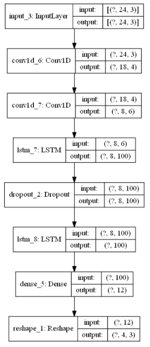
Vector Output Model

This architecture might be thought of as a much more common architecture compared to the above-mentioned models, however, it is not very suitable for our case. Nevertheless, I share an example model to give an idea. At variance with encoder-decoder architecture, neither RepeatVector nor TimeDistributed layer exists. The point is to add a Dense layer with FORECAST_RANGE*n_features node, and then reshape it accordingly at the next layer. You might also design a similar architecture with RepeatVector layer instead of Reshape layer.

The time steps of each series would be flattened in this structure and must interpret each of the outputs as a specific time step for a specific series during training and prediction. That means we also might reshape our label set as 2 dimensions rather than 3 dimensions, and interpret the results in the output layer accordingly without using Reshape layer. For simplicity, I did not change the shape of the label set, but just keep it in mind this alternative way as well. I also utilized Conv1D layers at the beginning of the architecture.

This structure might be also called a multi-channel model. Do not overestimate the names. When dealing with multiple time series, CNNs with multiple channels are utilized traditionally. In this structure, each channel corresponds to a single time series and similarly extracts convolved features separately for each time series. Since all of the extracted features are combined before feeding into the LSTM layer, some typical features of each time series might be lost.

input_layer = Input(shape=(LOOK_BACK, n_features)) 
conv = Conv1D(filters=4, kernel_size=7, activation=’relu’)(input_layer)
conv = Conv1D(filters=6, kernel_size=11, activation=’relu’)(conv)

lstm = LSTM(100, return_sequences=True, activation=’relu’)(conv)
dropout = Dropout(0.2)(lstm)
lstm = LSTM(100, activation=’relu’)(dropout)
dense = Dense(FORECAST_RANGE*n_features, activation=’relu’)(lstm)
output_layer = Reshape((FORECAST_RANGE,n_features))(dense)

model_vector_output = Model([input_layer], [output_layer])
model_vector_output.compile(optimizer=’adam’, loss=’mse’)

mae: 185.95
mse: 92596.76
mape: 9.49

Vector Output Model with CNN — Figure 6

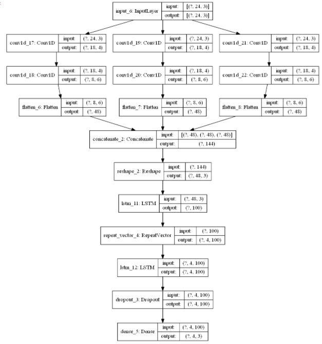
Multi-Head CNN-LSTM Model

This architecture is a bit different from the above-mentioned models. It is explained very clearly in the study of Canizo. The multi-head structure uses multiple one-dimensional CNN layers in order to process each time series and extract independent convolved features from each time series. These separate CNNs are called “head” and flattened, concatenated, and reshaped respectively before feeding into the LSTM layer. To summarize, multi-head structures utilize multiple CNNs rather than only one CNN like in multi-channel structure. Therefore, they might be more successful to keep significant features of each time series and make better forecasts in this sense.

input_layer = Input(shape=(LOOK_BACK, n_features)) 
head_list = []
for i in range(0, n_features):
 conv_layer_head = Conv1D(filters=4, kernel_size=7, activation=’relu’)(input_layer)
 conv_layer_head_2 = Conv1D(filters=6, kernel_size=11, activation=’relu’)(conv_layer_head)
 conv_layer_flatten = Flatten()(conv_layer_head_2)
 head_list.append(conv_layer_flatten)
 
concat_cnn = Concatenate(axis=1)(head_list)
reshape = Reshape((head_list[0].shape[1], n_features))(concat_cnn)

lstm = LSTM(100, activation=’relu’)(reshape)
repeat = RepeatVector(FORECAST_RANGE)(lstm)
lstm_2 = LSTM(100, activation=’relu’, return_sequences=True)(repeat)
dropout = Dropout(0.2)(lstm_2)
dense = Dense(n_features, activation=’linear’)(dropout)

multi_head_cnn_lstm_model = Model(inputs=input_layer, outputs=dense)

mae: 149.88
mse: 65214.09
mape: 8.03

Multi-Head CNN-LSTM — Figure 7

- Evaluation of the Model

Evaluation is basically the same with any forecasting modeling approach and the general performance of the models might be calculated with the evaluate_forecast method I shared in previous parts. However, there are 2 different points in our case, and it would be beneficial to take them into consideration as well. The first one is that we are performing multi-step forecasting, so we might want to analyze our forecasting accuracy for each of the time steps separately. This would give an insight into selecting an accurate forecast horizon. The second one is that we are performing a forecast for multiple parallel time series. Therefore, it would also be beneficial to observe the results of each time series forecasting. The model might work significantly worse for a specific time series than the rest of the time series.

You can simply utilize different kinds of evaluation metrics, I prefer Mean Absolute Percentage Error(mape) in this article that handles the different time series scales.

Given the stochastic nature of the models, it is good practice to evaluate a given model multiple times and report the mean performance on a test data set. For simplicity, I just run them only once in this article.

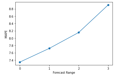
With respect to each time step output, I just share a simple code snippet and figure that represents the mape values of forecasting for each time step. As expected, mape increases along with an increasing forecasting range. The figure represents the Multi-Head CNN-LSTM architecture and might be applied directly to other architectures I mentioned above. If you observe a sharp increase in mape, you might decrease your forecast horizon and set it to the point just before the sharp increase.

y_test_inverse_time_step = y_test_inverse.reshape(int(y_test_inverse.shape[0]/FORECAST_RANGE), FORECAST_RANGE, y_test_inverse.shape[-1])

yhat_inverse_time_step = yhat_inverse.reshape(int(yhat_inverse.shape[0]/FORECAST_RANGE), FORECAST_RANGE, yhat_inverse.shape[-1])

# yhat_inverse_time_step and y_test_inverse_time_step are both same dimension.
time_step_list_yhat = [[] for i in range(FORECAST_RANGE)]
time_step_list_y_test = [[] for i in range(FORECAST_RANGE)]

for i in range(0, yhat_inverse_time_step.shape[0]):
 for j in range(0, yhat_inverse_time_step.shape[1]):
 time_step_list_yhat[j].append(list(yhat_inverse_time_step[i][j]))
 time_step_list_y_test[j].append(list(y_test_inverse_time_step[i][j]))

yhat_time_step = np.array(time_step_list_yhat)
yhat_time_step = yhat_time_step.reshape(yhat_time_step.shape[0], -1)
y_test_time_step = np.array(time_step_list_y_test)
y_test_time_step = y_test_time_step.reshape(y_test_time_step.shape[0], -1)

# plotting
mape_list = []
for i in range(0, FORECAST_RANGE):
 mape = mape_(y_test_time_step[i], yhat_time_step[i])
 mape_list.append(mape)

plt.plot(range(0, FORECAST_RANGE), mape_list, marker=’o’)
plt.xticks((range(0, FORECAST_RANGE)))
plt.xlabel(‘Forecast Range’)
plt.ylabel(‘MAPE’)

Forecasting Range vs MAPE — Figure 8

The following code snippet might be used for analyzing model performance with respect to different input time series. The forecast performance of the model is better for all CPUs compared to the overall results of the baseline model. Although mae of the second CPU is significantly low compared to the other CPUs, its mape is significantly higher than the others. Actually, it is one of the reasons why I am using mape in this article as an evaluation criterion. Each of the CPU usage values behaves similarly, but completely on different scales. To be honest, it has been a good example of my point. Why error ratio for the second CPU is so high? What should I do in such circumstances? Dividing the entire time series into subparts, and developing separate models for each of them might be an option. What else? I really appreciate reading any valuable approaches in the comments.

Even though it is not very meaningful for our case, plotting a histogram for the performance of each time series would be expressive for data sets including more parallel time series.

for i in range(0, n_features):
 print(‘->‘, i)
 mae = mae_(y_test_inverse[:,i],yhat_inverse[:,i])
 print('mae:', mae)
 mse = mse_(y_test_inverse[:,i],yhat_inverse[:,i])
 print('mse:', mse)
 mape = mape_(y_test_inverse[:,i],yhat_inverse[:,i])
 print('mape:', mape)

-> 0
mae: 126.53
mse: 32139.92
mape: 5.44
-> 1
mae: 42.03
mse: 3149.85
mape: 13.18
-> 2
mae: 281.08
mse: 160352.55
mape: 5.46

- Final Words

Before finalizing the article, I want to touch on a few important points about time series forecasting in real life. First of all, traditional methods used in machine learning for model evaluation are mostly not valid in time series forecasting. It is because they do not take into consideration temporal dependencies that are the case for time series.

3 different methodologies are mentioned here. The most straightforward one is to determine a split point and separate the data set as train and test without shuffling just as we have done in this article. However, in real life, it does not give a robust insight into the performance of the model.

The other one is to repeat the same strategy multiple times, that is multiple train test splits. In this method, you create multiple train and test sets and so multiple models. You should consider keeping the test set size the same to compare the models' performance correctly. You might also keep the train set size the same by only taking into account a fixed length of the latest data. Note that there is a package in sklearn called as TimeSeriesSplit to perform this methodology.

The final most robust methodology is walk forward validation which is the k-fold cross-validation of the time series world. In this approach, a new model is created after each forecast by including new known value to the train set. It is repeated continuously with a sliding window approach and takes into a minimum number of observations for training the model. It is the most robust method but comes with a cost obviously. To create many models for especially mass amounts of data might be cumbersome.

Apart from the traditional ML approaches, time series forecasting models should be updated more frequently in order to capture changing trend behaviors. However, in my opinion, the model does not need to be retrained whenever you want to generate a new prediction as stated here. It will be very costly and unnecessary if the time series does not change in a very frequent and drastic way. What I agree totally with the above article is that accurately defining confidence intervals for forecasting is as important as forecasting itself, even more important in real-life scenarios considering anomaly detection use cases. It deserves to be the topic of another article.

Last but not definitely least, running a multi-step forecasting model in production is quite different from traditional machine learning approaches. There are a few options, the most common ones are recursive and direct strategies. In recursive strategy, at each forecasting step, the model is used to predict one step ahead and the value obtained from the forecasting is then fed into the same model to predict the following step. The same model is used for each forecast. However, at this strategy, the forecasting error propagates along the forecast horizon as you can expect. And it might be a burden, especially for long forecast horizons. On the other hand, a separate model is designed for each forecast horizon in direct strategy. It will be obviously overwhelmed with the increasing length of the forecast horizon, which means an increasing number of models. Furthermore, it does not take into account statistical dependencies among the predictions since each model is independent of each others. As another strategy, you might also design a model that is capable of performing multi-step forecasting at once like what we did in this article.

In this article, I focus on a very specific use case for time series forecasting but a common use case at the same time in real-life scenarios. Additionally, I mention a few general key points that should be taken into consideration while implementing forecasting models.

When you encounter multiple time series and are supposed to perform multi-step forecasting for each of them, firstly try to create separate models to achieve the best result. However, the number of time series might be extremely much in real life, you should also consider using above mentioned single model architectures in such cases. You might also utilize different kinds of layers like Bidirectional, ConvLSTM adhering to the architectures, and get better results by tuning parameters. The use cases I mention mostly consist of the same unit time series like traffic values flowing through each device or temperature values of different devices spread over a large area. To see the results with different kinds of time series would be interesting as well. For instance, a single model approach for forecasting temperature, humidity, pressure at once. I believe it is still an open research area considering lots of different academic studies in this area. In this sense, I appreciate hearing different approaches as well in the comments.

USEFUL LINKS

• Multi-head CNN-RNN for multi-time series anomaly detection: An industrial case study
• Ensemble of Multi-headed Machine Learning Architectures for Time-Series Forecasting of Healthcare Expenditures
• A study of deep learning networks on mobile traffic forecasting
• Multi-Step LSTM Time Series Forecasting Models for Power Usage - Machine Learning Mastery
• How to Develop LSTM Models for Time Series Forecasting - Machine Learning Mastery
• Time Series Forecasting

---

CNN-LSTM based Models for Multiple Parallel Input and Multi-Step Forecast was originally published in Towards Data Science on Medium, where people are continuing the conversation by highlighting and responding to this story.

from Towards Data Science - Medium https://ift.tt/2YUPRgv
via RiYo Analytics