https://ift.tt/3CVNuYS The lesser known type of quantum computers that are easier to build, easier to understand, and (maybe) equally as po...
The lesser known type of quantum computers that are easier to build, easier to understand, and (maybe) equally as powerful.
I’ve just completed my thesis for Honours at the Australian National University, which proposed how diamonds could be used as adiabatic quantum computers. During this project however, I realised that there are few people with any idea what adiabatic quantum computers, even within the quantum computing field more broadly.
This series aimed at quantum beginners with some Python skills (to be published weekly) attempts to explain what it is through a computational lens, with each article also being a notebook that can be executed on Deepnote and linked at the top. The Series will proceed as follows
- Foundational knowledge and what the whole endeavour relies on: the Adiabatic Theorem.
- Building a model for computation using the Quadratic Unconstrained Binary Optimisation framework, and an isomorphism to the Ising model.
- The most important constraint: Qubit Connectivity, mathematical graphs and the minor embedding problem.
- Simulating ideal and noisy adiabatic quantum computers, and running some experiments.
- Discussing the debates around computational complexity, quantum speedup, and my opinions on the future of the space (and insights into my research)
Let’s dive in!
Quantum Computing is a hot topic at the moment, with promises to revolutionize encryption, enable the discovery of new drugs, and push the barriers for machine learning. To make these promises reality, there are two fundamentally different approaches to achieving quantum computing. These are
- Gate-based Quantum Computing
If you have basic familiarity with quantum computing, this is almost certainly what you read about. This is the approach which has the famous Shor’s algorithm for prime number factorization (break encryption), and Grover’s search algorithm. Furthermore, this is the approach currently being invested in by Google, IBM, Honeywell, etc. Gate-based quantum computers should be thought about in the same way as current classical computers, where it performs a series of transformations (logic gates) to arrive at a specific conclusion. I wil call this type of approach digital computing.
2. Adiabatic Quantum Computing
The focus of this series is the other, less well-known type of quantum computing. Conversely to gate-based approaches, adiabatic quantum computers are analog computers. I think the best way to describe analog computation is through analogy. Imagine you wanted to add two sound waves together. A digital approach would involve finding a discrete encoding of the sound signals, and writing an algorithm in a programming language that adds the two waves together at each point in time. However, you could construct a physical analog of the problem by simply finding two speakers, and playing the sound waves through the speakers. Then, the fluid dynamics (or whatever physics) of playing waves through a medium does the computation for you, and you just record the result.
The problems that can already (in theory) be solved using an adiabatic quantum computer are the Travelling Salesman Problem, the Maximum Cut problem, and many other extremely challenging combinatorial optimisation problems.
In this series, I will try to avoid talking about any quantum mechanics unless absolutely necessary.
The Adiabatic Theorem
The whole foundation of adiabatic quantum computing is the adiabatic theorem (of quantum mechanics). In the formulation most useful to us, it states that
- if a quantum state is initialised into the ground state of a system, then any small enough changes to that system will (with high probability) keep it in the ground state.
This allows for a very simple procedure for any adiabatic computation
- Initialise the state into the ground state of an easy to implement initial system
- Design a target system where the ground state encodes the solution to some interesting problem
- Transition from the initial system to the target system slowly enough that all changes are small, and end up in the ground state of the target system
- Read out the final state, which should be the ground state that was constructed to be the solution to your problem
For the code of this article, I want to demonstrate each of the following important concepts
- The evolution of a quantum state in a specific system through the Schrodinger equation
- How transitioning from an initial system to a final system quickly excites the quantum state into many higher energy states
- How transitioning from an initial system to a final system slowly keeps most of the quantum probability in the ground state.
Alright, now let’s dive into the code parts!
You should absolutely feel free to skip past some of the finer details here
Set up
Since we are working using a numerical simulation we discretize position and momentum of the space.
Now we want to transition from an initial system to a target system. ‘Systems’ in quantum mechanics are ways to identify the energy of a certain state, and are called Hamiltonians. For this example, we will use one of the simplest Hamiltonians, which is a quadratic of the form

This gives the well-studied Quantum Harmonic Oscillator( which has analytic solutions for the states.
Recalling that we want to transition from an initial state to a final state over some time we write

Simulating the Schrödinger evolution
Quantum systems evolve according to the Schrödinger Equation, which is a partial differential equation. For the physicists reading, note that here I use natural units (ℏ=1)

Since I want to simulate this numerically, I will need to use a method for integrating PDEs. I used the Split Step Fourier method, for which I found a tutorial using the Schrödinger Equation
Functions required for split-step Fourier method can safely be used for an arbitrary 1-D potential if you want to have a play with this yourself.
What I want to show
I want to transition from an initial potential V_i to V_T for two different values of t_total. One quickly (where many excited states happen), and one slowly where most of the probablity stays in the ground state. I want to show that the majority of the probability remains in the ground state over the slow evolution..
Note that the right hand side bar charts show how ‘ground-statey’ or ‘excited-statey’ a particular wavefunction is. Whilst people who have done quantum physics will know what this means, it actually makes way more sense to delay introducing this properly until next week’s article. For the lay-reader who is approaching this for the first time, the larger the bars on the left, the better, because it’s a measure of how likely the ground state is, which is what we wanted in our construction at the start.
The slow evolution
As we evolve slowly from our initial potential/Hamiltonian/system to our target Hamiltonian we see that the vast majority of probability remains in the ground state, as shown by the bar chart on the left. We can see that this is achieved because only minimal change is required to follow along the potential. If you increase max_t and t_total even further, this will continue to be an even better approximation.
Animating that (code can be found in the notebook) shows
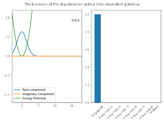
During the entire evolution the vast majority of the probability remains in the ground state, with only tiny excitations required to cause the wavefunction to to remain in the ground state. Note that here the ground state is defined with respect to the instantaneous ground state of the potential.
The fast evolution
Conversely, we can immediately see that following the exact same procedure, but changing the potential 3x faster causes there to be large excitations into the excited states. This violates the adiabatic condition of changing slow enough, and means that this would not be useful in an adiabatic quantum computation.

Conversely, we see that with a faster transition, there is a much smaller amount of ‘ground-stateness’ in the wave-function. This would mean that this was significantly too fast for useful adiabatic computation.
What you should take away
This first dip in the waters of quantum mechanics and the adiabatic theorem should have shown you that
- If you can start in the ground state of a system, then evolving slowly means that you will mostly stay in the ground state
- We can ‘trade-off’ the strength of two systems by simultaneously increasing the strength (prefactor) of one whilst turning the other down, allowing for a completely general way of achieving slow evolution
- This allows for a single, generic construction of doing computation as long as we could figure out how to encode the solution of a problem into the ground state.
What we’ll cover next week
- Moving to qubits which have binary values
- Producing the exact constructions required to encode the solution of a problem into the ground state.
Running the code written here
I wrote all of this code using an online Jupyter Notebook editor Deepnote, if you click here you can see this article published there, and click the “Launch in Deepnote” button to copy the notebook and run it from scratch yourself!
Feel free to reach out and give feedback on this style of writing, and to ask any questions you have so that I can address them in next weeks installment!
Adiabatic Quantum Computation 1: Foundations and the Adiabatic Theorem was originally published in Towards Data Science on Medium, where people are continuing the conversation by highlighting and responding to this story.
from Towards Data Science - Medium https://ift.tt/3HT8vqO
via RiYo Analytics


No comments