https://ift.tt/3CUp8iS How they work, and why they are 'Hidden’. A Hidden Markov Model can be used to study phenomena in which only a ...
How they work, and why they are 'Hidden’.
A Hidden Markov Model can be used to study phenomena in which only a portion of the phenomenon can be directly observed while the rest of it cannot be directly observed, although its effect can be felt on what is observed. The effect of the unobserved portion can only be estimated.
We represent such phenomena using a mixture of two random processes.
One of the two processes is a ‘visible process’. It is used to represent the observable portion of the phenomenon. The visible process is modeled using a suitable regression model such as ARIMA, the Integer Poisson model, or the ever popular Linear Model. The portion that cannot be observed is represented by a ‘hidden process’ which is modeled using a Markov process model.
If you are new to Markov processes, please read the following article and then come back here to continue reading:
A Beginner’s Guide to Discrete Time Markov Chains
A real word illustration of a Hidden Markov Model
Let’s illustrate how a Hidden Markov Model can be used to represent a real world data set.
The following graphic shows the monthly unemployment rate in the United States:
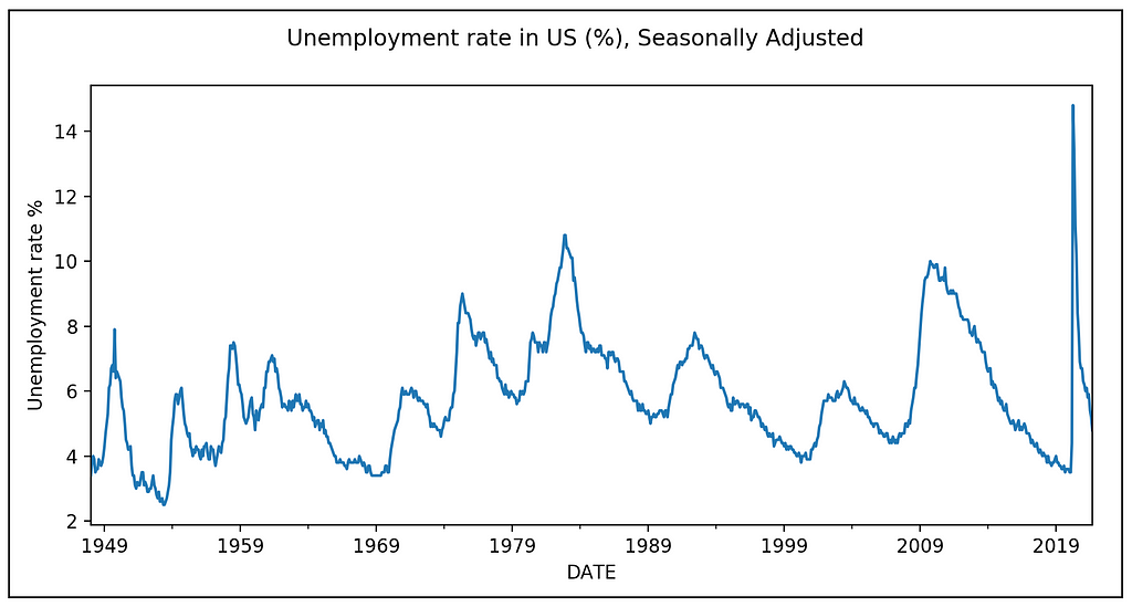
The above graph shows large scale regions of positive and negative growth. We hypothesize that there is some hidden process at play that is unbeknownst to the observer, flip-flopping between two ‘regimes’ and the current regime in effect is influencing the observed trend in the inflation rate.
While modeling the above data set, we will consider a regression model that is a mixture of the following two random variables:
- The observable random variable y_t, which would be used to represent the observable pattern in unemployment rate. At each time step t, y_t is simply the observed value of the unemployment rate at t.
- A hidden random variable s_t which is assumed to change its state or regime, and each time the regime changes, it affects the observed pattern of employment. In other words, a change in value of s_t impacts the mean and variance of y_t. This is the primary idea behind Hidden Markov Models.
We’ll see how to precisely express this relationship between y_t and s_t. For now, let’s assume that s_t switches between two regimes 1 and 2.
The important question is: why are we calling s_t a ‘hidden’ random variable?
We call s_t hidden because we do not know exactly when it changes its regime. If we knew which regime was in effect at each time step, we would have simply made s_t a regression variable and we would have regressed y_t on s_t!
Formulation of the hidden random variable s_t
For the unemployment data set, we will assume that s_t obeys a 2-state Markov process having the following state transition diagram:
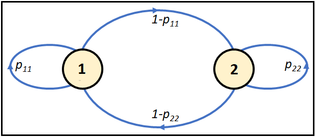
The Markov chain shown above has two states, or regimes numbered as 1 and 2. There are four kinds of state transitions possible between the two states:
- State 1 to state 1: This transition happens with probability p_11.
Thus p_11= P(s_t=1|s_(t-1)=1). This is read as the probability that the system is in regime 1 at time t, given that it was in regime 1 at the previous time step (t-1). - State 1 to State 2 with transition probability:
p_12= P(s_t=2|s_(t-1)=1). - State 2 to State 1 with transition probability:
p_21=P(s_t=1|s_(t-1)=2). - State 2 to State 2 with transition probability:
p_22= P(s_t=2|s_(t-1)=2).
Since the Markov process needs to be in some state at each time step, it follows that:
p11 + p12 = 1, and,
p21 + p22 = 1
The state transition matrix P lets us express all transition probabilities in a compact matrix form as follows:
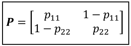
P contains the probabilities of transition to the next state which are conditional upon what is the current state.
The state probability vector π_t contains the unconditional probability of being in a certain state at time t. For our 2-step Markov random variable s_t, the state probability distribution π_t, (a.k.a. δ_t) is given by the following 2-element vector:

It can be shown that if we start with some prior (initial) probability distribution for s_t as π_0, then π_t can be computed by simply matrix multiplying P with itself t number of times and multiplying π_0 by the matrix product P^t:

We have thus completed the formulation of the Markov distributed random variable s_t. Recollect that we are assuming s_t to be the hidden variable.
Let’s pause for a second and remind ourselves of two important things that we do not know:
- We do not know the exact time steps at which s_t makes the transition from one state to another.
- We also do not know the transition probabilities P or the state probability distribution π_t.
Therefore, what we have done so far is to hypothesize that there exists a two-regime Markov process characterized by the random variable s_t, and s_t is influencing the observed unemployment rate which is characterized by the random variable y_t.
Formulation of the observable time series variable y_t
For a second, let’s assume that there is no hidden Markov process influencing the unemployment rate y_t. And with that assumption, let us construct the following regression model for the unemployment rate y_t:
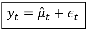
We are saying that at any time t, the observed unemployment rate y_t is the sum of the modeled mean μ_cap_t and the residual error ε_t. The modeled mean μ_cap_t is the regression model’s prediction of unemployment rate at time t. The residual error ε_t is simply the predicted rate subtracted from the observed rate. We’ll use the terms modeled mean and predicted mean interchangeably.
We will further assume that we have used a really good regression model to calculate the modeled mean μ_cap_t. And therefore, the residual error ε_t can be assumed to be homoskedastic i.e. its variance does not vary with the mean, and furthermore, ε_t is normally distributed around a zero mean and some variance σ². In notation form, ε_t is an N(0, σ²) distributed random variable.
Let us now return to μ_cap_t. Since μ_cap_t is the predicted value of the regression model, μ_cap_t is actually the output of some regression function η(.) such that:
μ_cap_t = η(.)
Different choices of η(.) will yield different families of regression models.
For example, if η(.) = 0, we get the white noise model: y_t = ε_t.
If η(.) is the constant mean y_bar of all observations i.e.:
y_bar=(y_1+y2+…+y_n)/n,
we get a mean model: y_t = y_bar.
A more interesting model might rely upon a set of ‘m+1’ number of regression coefficients β_cap=[β_cap_0, β_cap_1, β_cap_2, …, β_cap_m] that ‘link’ the dependent variable y to a matrix of regression variables X of size [n X (m+1)] as illustrated below:
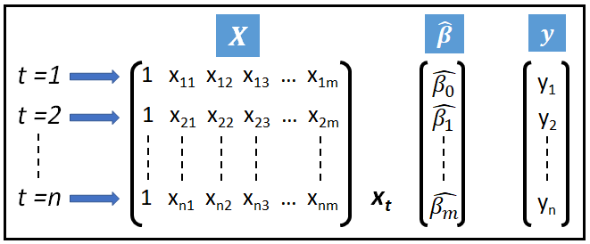
In the above figure, the first column of ones in X acts as the placeholder for the fitted intercept of regression β_cap_0. The ‘cap’ symbol signifies that it is the fitted value of the coefficient after training the model. And x_t is one row of X at time t.
If the link function η(x_t, β_cap) is linear, one gets the Linear model.If the link function is exponential, one gets the Poisson, NLS etc. regression models and so on.
Let’s take a closer look at the Linear Model, characterized by the following set of equations:

At the risk of making the residual errors ε_ t correlated, one is also allowed to introduce lagged values of y_t in x_t, as follows:

In case you are wondering, no, the above model is not an Auto-Regressive model in the ARMA sense of that term. Later, we will look at how a ‘real’ AR(1) model looks like.
Our model specification isn’t complete unless we also specify the probability (density) function of y_t. In the above model, we will assume y_t to be normally distributed with mean μ_cap_t, and constant variance σ²:

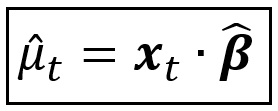
The above equation is to be read as follows: The probability (density) of the unemployment rate being y_t at time t, conditioned upon the regression variables vector x_t and the fitted coefficients vector β_cap is normally distributed with a constant variance σ² and a conditional mean μ_cap_t given given by the equation below:
This completes the formulation of the visible process for y_t.
Now let’s ‘mix’ the hidden Markov process and the visible process into a single Hidden Markov Model.
Mixing the hidden Markov variable s_t with the visible random variable y_t
The key to understanding Hidden Markov Models lies in understanding how the modeled mean and variance of the visible process are influenced by the hidden Markov process.
We will introduce below two ways in which the Markov variable s_t influences μ_cap_t and σ².
The Markov Switching Dynamic Regression (MSDR) model
Suppose we define our regression model as follows:

In the above equation, we are saying that the predicted mean of the model changes depending on which state the underlying Markov process variable s_t is in at time t.
As before, the predicted mean μ_cap_t_s_t can be expressed as the output of some link function η(.), i.e. μ_cap_t_s_t = η(.).
For this model, we define η(.) as follows:
![The predicted mean expressed as a dot product of a vector of 1s of size [n x 1] and a vector of coefficients of size [1 x 1]](https://cdn-images-1.medium.com/max/539/1*pDtU2Ix_N_bMtR25wjIyAA.png)
The above equation is a special simple case of the dot product x_t·β_cap, where there are no regression variables involved. So x_t is a matrix of size [1 X 1] containing the number 1 which as we have seen earlier, is the placeholder for the intercept of regression β_0. β_cap is also a [1 x 1] matrix containing only the intercept of regression β_0_s_t. The dot product of the two is the scalar value β_0_s_t which is the value that the intercept takes under the Markov regime s_t at time t.
If we assume that the Markov process operates over the set of k states [1,2,3,…j,…,k], it is easier to express the above equation as follows:

And the regression model’s equation becomes the following:

In the above equation, y_t is the observed value, μ_cap_t_j is the predicted mean when the Markov process is in state j, and ε_t is the residual error of regression.
In our unemployment rate data set, we have assumed that s_t toggles between two regimes 1 and 2, which gives us the following specification for μ_cap_t_j:

This in turn gives rise to a mixture process for y_t that switches between two means μ_s_1 and μ_s_2 as follows:

The corresponding two conditional probability densities of y_t are as follows:

But each observed y_t ought to have only one probability density associated with it.
We will calculate this single density using the Law of Total Probability which states that if event A can take place pair-wise jointly with either event A1, or event A2, or event A3, and so on, then the unconditional probability of A can be expressed as follows:

Here’s a graphical way of looking at it. There are ’n’ different ways of reaching node A:
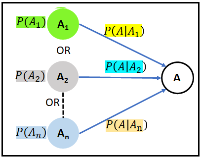
Using this law, we get the unconditional probability density of observing a specific unemployment rate y_t at time t as follows:

The astute reader may have noticed that in the above equation we are mixing probabilities with probability densities, but it is okay to do that here. The above equation written in summation form is as follows:

In the above equation, the probabilities P(s_t=1) and P(s_t=2) are the state probabilities π_t1 and π_t2 of the 2-state Markov process:

And we already know that to calculate the state probabilities, we need to assume some initial conditions and then use the following equation:

Where π_0 is the initial value t=0, and P is the state transition matrix:

The above model is a simple case of what’s known as the Markov Switching Dynamic Regression (MSDR) family of models.
Estimation and training
Training this model involves estimating the optimal values of the following variables:
- The state transition matrix P, i.e. essentially, transition probabilities p_11 and p_22,
- The state specific regression coefficients β_cap_0_1 and β_cap_0_2, which in our sample data set would correspond to the two predicted unemployment rate levels, and,
- The constant variance σ².
Estimation can be done using Maximum Likelihood which finds the values of P, β_cap_0_1, β_cap_0_2 and σ² that would maximize the joint probability density of observing the entire training data set y. In other words, we would want to maximize the following product:
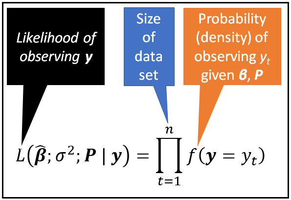
In the above product, the probability density f(y=y_t) is given by Equation (1) that we saw earlier.
It is usually easier to maximize the natural logarithm of this product which has the benefit of converting products into summations. Hence we maximize the following log-likelihood:

Maximization of Log-Likelihood is done by taking partial derivatives of the log-likelihood w.r.t. each parameter p_11, p_22, β_cap_0_1, β_cap_0_2 and σ² , setting each partial derivative to zero, and solving the resulting system of five equations using some optimization algorithm such as Newton-Raphson, Nelder-Mead, Powell’s etc.
Markov Switching Dynamic Regression model (the general case)
The general equations of the MSDR can be stated as follows:

Where, μ_cap_t_j is a function of regression variables matrix x_t and regime-specific fitted coefficients matrix β_cap_s. i.e.,
μ_cap_t_j = η(x_t, β_cap_s)
If the Markov model operates over ‘k’ states [1,2,…,j,…,k], β_cap_s is a matrix of size [k X (m+1)] as follows:
![The coefficients matrix of size [k x (m+1)]](https://cdn-images-1.medium.com/max/524/1*YDkdy7xZv9Jp2QrO0lS6rw.png)
The central idea is that depending on which one of the regimes j in [1, 2,…,k] is currently in effect, the regression model coefficients matrix β_cap_s will switch to the appropriate regime-specific vector β_cap_j.
The k-state Markov process itself is governed by the following state transition matrix P:
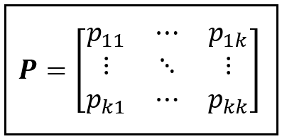
And it has the following state probability distribution π_t at time step t:

So far, we have assumed a linearly specified conditional mean function for y_t as follows:

In the above equation, μ_cap_t_j is the predicted mean at time t under Markov regime j. x_t is the vector of regression variables [x_1t, x_2t,…,x_mt] at time t, and β_cap_j is the vector of regime specific coefficients [β_cap_0j, β_cap_1j, β_cap_2j,…,β_cap_mj].
As we have seen in the 2-state Markov case (refer to Eq. 1), this yields a normally distributed probability density for y_t as follows:

Equation (2) is just Equation (1) extended over k Markov states.
y_t need not be normally distributed. In fact, suppose y_t represents a whole numbered random process i.e. y_t takes values 0,1,2,…etc. Examples of such processes are the number of motor vehicle accidents per day in New York City, or hourly number of hits on a website. Such processes can be modeled using a Poisson process model. In which case, the Probability Mass Function of a Poisson distributed y_t takes the following form:

Where the regime specific mean function is expressed as follows:

In the above equation, x_t and β_cap_j have the same meaning as with the linear mean function.
Training and estimation
Training of the Markov Switching Dynamic Regression model involves the estimation of the optimal values of the following variables:
The model’s coefficients:
![The coefficients matrix of size [k x (m+1)]](https://cdn-images-1.medium.com/max/524/1*YDkdy7xZv9Jp2QrO0lS6rw.png)
The state transition probabilities:

and variance σ².
As before, the estimation procedure can be Maximize Likelihood Estimation (MLE) in which we are solving a system of (k² +(m+1)*k +1) equations (in practice, much fewer than that number) corresponding to k² Markov transition probabilities, (m+1)*k coefficients in β_cap_s, and the variance σ².
In an upcoming article, we’ll look at how to build and train both Linear and Poisson MSDR models using Python and the statsmodels library.
Let’s now look at another type of Hidden Markov Model known as the Markov Switching Auto Regressive (MSAR) model.
The Markov Switching Auto Regressive (MSAR) model
Consider the following model equation for the monthly unemployment rate:

Here, we are saying that the unemployment rate at time t fluctuates around a regime specific mean value μ_t_s_t. The fluctuation is caused by the sum of two components:
- The first component represents the fraction of the deviation of the observed value at the previous time step from the fitted regime-specific mean at the previous time step, and,
- The second component comes from the residual error ε_t.
As with the MSDR model, the regime of the hidden Markov process influences the fitted mean of the model.
Notice that this model depends not only on the value of the regime at time t but also on what regime was in effect at the previous time step (t-1).
The above specification can be easily extended to include p time steps in the past so to get an MSAR model that follows the AR(p) design pattern.
Model specification and estimation
The general framework for model specification for the MSAR model, including the specification of the probability density function of y_t and the estimation procedure (MLE or Expectation Maximization) remains the same as with MSDR model.
Unfortunately, the dependence of the model on Markov states at previous steps considerably complicates the specification process as well as estimation.
We will not get into those details here, but as with the MSDR model, we will look at how to build and train an MSAR model in Python and statsmodels in an upcoming article.
References and Copyrights
Data set
U.S. Bureau of Labor Statistics, Unemployment Rate [UNRATE], retrieved from FRED, Federal Reserve Bank of St. Louis; https://ift.tt/3kXQG0R, October 29, 2021. Available under Public license.
Books
Cameron A. Colin, Trivedi Pravin K., Regression Analysis of Count Data, Econometric Society Monograph №30, Cambridge University Press, 1998. ISBN: 0521635675
James D. Hamilton, Time Series Analysis, Princeton University Press, 2020. ISBN: 0691218633
Images
All images are copyright Sachin Date under CC-BY-NC-SA, unless a different source and copyright are mentioned underneath the image.
Related reads
- A Beginner’s Guide to Discrete Time Markov Chains
- An Introduction to the Poisson Integer ARIMA Regression model
- Poisson Regression Models for Time Series Data Sets
- An Illustrated Guide to the Poisson Regression Model
Thanks for reading! If you liked this article, please follow me to receive tips, how-tos and programming advice on regression and time series analysis.
A Math Lover’s Guide to Hidden Markov Models was originally published in Towards Data Science on Medium, where people are continuing the conversation by highlighting and responding to this story.
from Towards Data Science - Medium https://ift.tt/3mYwOvf
via RiYo Analytics

No comments