https://ift.tt/3jfmYm4 Understanding Bias-Variance Tradeoff from the equation Many of us have read about the Bias and Variance at various ...
Understanding Bias-Variance Tradeoff from the equation
Many of us have read about the Bias and Variance at various places in the AI literature but still many people struggle to explain it with respect to mathematical equation. People always comment about bias-variance whenever they build a model in order to figure out whether the model can be used or not in the real world and how good its performance will be. In this article, we will focus on the mathematical equation depicting Bias-Variance and try to understand different parts of this equation from a mathematical perspective. Let me first highlight some of the assumptions that are essential in order to understand the equation:
Assumptions
- There is a Hypothesis set H that we are using while training a model.
- There is an actual target function f that we try to approximate using the learning algorithm and the dataset D. This function f is always unknown.
- When we take a dataset D and apply a learning algorithm over it, we will get a prediction function g, that tries to approximate the actual target function f.
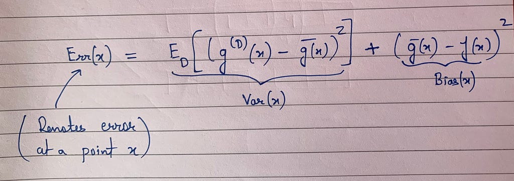
- There is a datapoint x that belongs to the dataset D.
We will be using above assumptions in the equation below.
As the main focus of this article is to understand the bias-variance equation from mathematical perspective, we will directly look at the equation without going into the derivation behind it(Please check the references, if you want to understand the derivation).
Before delving into the explanation, let’s first look at the equation of Bias and Variance:
Explanation
In the above equation, we assume that we are looking at a data point x and finding out the error. Now in order to understand the right hand side, we use the above mentioned assumptions. Let’s say we have a hypothesis set H(which indicates the class of functions that we can probably go over while training). Now let’s say we apply the learning algorithm by taking the dataset D and running empirical risk minimization(training a model using an optimization algorithm to minimize empirical loss) over the same to get a predictor function g. In the above equation the g^D(x) indicates that g is explicitly attached to the dataset D because with different realizations of a dataset D, we will get different predictor functions. For example: let’s say we have 10 different realizations of a dataset D as: D1, D2, D3,…..,D10. Now when we take each of them and run empirical risk minimization, we will get different predictors as g1, g2, g3, ……,g10 respectively. Note that I have taken only 10 datasets and corresponding to that there are 10 different predictors just for the sake of explaining but there can be infinitely many realizations.
Now imagine we have many different predictors indicated by g_i and we take the average of them to get g^bar(x). Mathematically speaking g^bar(x) can be shown to be somewhat better as compared to other learned predictors and is more closer to the actual target function f. Now the first part of the right hand side in above equation simply indicates the variance of predictor function g^D(x). With the single realization of dataset D(which simply means that the dataset which we explicitly have with us or is given to us) we will get some predictor g^D(x) and we measure the spread of different predictors around the average predictor g^bar(x) that simply indicates the variance.
Understanding the second part of the above equation is quite simple, we are trying to measure how far the prediction of our best average predictor g^bar(x) is with respect to the actual target function f(x). This difference indicates the bias in our prediction for a datapoint x.
Now practically speaking while we train a model and measure the error, we never have access to this average predictor as well as the actual target function, what we have is some dataset that we are trying to use to train the model and some hypothesis set based upon our modelling decisions. let’s say we choose hypothesis set as neural networks to train over the given dataset. After training, we will get some predictor function g^D(i.e., a neural network) using which we can measure the error over the datapoints in our test set. And theoretically whatever error we will measure will have some portion of it that will be attributed to bias and some portion to variance and also there is some irreducible error that is not shown in the above equation.
After looking at the above equation, we can quickly relate the concepts like overfitting in which whenever we see that the training error is very low but test error is high, we quickly say that it is overfitting and it is a case of low bias and high variance. Here low bias indicates that the average predictor is very close to the actual target function f. And high variance is indicative of the fact that predictors in our hypothesis set are too much spread out with respect to the average predictor, i.e., g^bar(x) meaning with different dataset I will obtain different predictor and they are not close to each other. So, in order to resolve such a situation we quickly start applying regularization techniques which theoretically reduces the size of the hypothesis set by putting constraints(try to relate L1 and L2 regularization formulation ) over the model parameters. Intuitively speaking, due to these constraints as the hypothesis set gets reduced the variance start getting reduced but again the bias starts getting increased. And the reason for an increased bias is the fact that since we have a restricted hypothesis set, the average predictor will now change and will depend only on those predictors that are present in the reduced hypothesis set due to which its closeness with respect to actual target function f might decrease which will result in increased bias.
Note
When you see the bias-variance equation in the literature there is another expectation over the data points x which simply indicates that we report the expected error over all the data points in the test set but in this article we simply tried understanding the equation with respect to one data point.
If you want to deep dive further and see how the equation is derived, feel free to look at the references:
References
https://www.youtube.com/watch?v=zrEyxfl2-a8&list=PLD63A284B7615313A&index=8
Mathematical Understanding of Bias Variance Tradeoff was originally published in Towards Data Science on Medium, where people are continuing the conversation by highlighting and responding to this story.
from Towards Data Science - Medium https://ift.tt/2Z2e5pr
via RiYo Analytics


ليست هناك تعليقات