https://ift.tt/3jkcVMP Mapping books to different slots on the shelf. Photo by Sigmund on Unsplash How to design data representation t...

How to design data representation techniques with applications to fast retrieval tasks
Hashing is one of the most fundamental operations in data management. It allows fast retrieval of data items using a small amount of memory. Hashing is also a fundamental algorithmic operation with rigorously understood theoretical properties. Virtually all advanced programming languages provide libraries for adding and retrieving items from a hash table.
More recently, hashing has emerged as a powerful tool for similarity search. Here the objective is not exact retrieval but rather the fast detection of objects that are similar to each other. For example, different images of the same item should have similar hash codes, for different notions of similarity, and we should be able to search fast for such similar hash codes.
A recent research trend has been the design of data-specific hash functions. Unlike the traditional algorithmic approach to hashing, where the hash functions are universal and do not depend on the underlying data distribution, learning to hash approaches are based on the premise that optimal hash functions can be designed by discovering hidden patterns in the data.
In this post, I will discuss machine learning techniques for the design of data-specific hash functions and their applications.
Data distribution hashing
This is the standard hashing, for example, dictionaries in Python where we store key, value pairs. The keys are mapped to unique hash codes and we can retrieve in constant time if a key is present in our hash table or dictionary.
Data independent (traditional) hashing
We assume that items, or keys, are represented by integer numbers. (Immutable data types such as strings, floats, or tuples can be represented as integers.)
The standard hashing approach is to map an item x to f(x) where f(x) can only take one of m distinct values. It is important that the f(x) values are as random as possible, i.e. we want

In this way, we are less likely to have collisions, i.e., f(x)=f(y). Collisions are usually handled by creating a list containing all items hashed to a given address. If the list is too long, the retrieval becomes slow as we need to traverse the list.
In order to avoid collisions, the hash function should be independent:
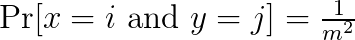
for all inputs and 0 ≤ i, j ≤ m-1.
The above condition is called 2-wise independence because we consider the independence only for pairs of input items. If we had triples of items, we would have 3-wise independence, and in general k-wise independence. The higher k, the more random the function.
One of the main requirements for hash functions is that they can be efficiently evaluated. A typical example is a linear hash function like
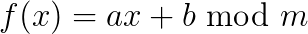
where a and b are randomly selected prime numbers. One can show that this function is 2-wise independent. More complex functions such as higher degree polynomials yield k-wise independence for k>2. The trade-off is that more complex functions are also slower to evaluate. I refer to these lecture notes for more details on hashing.
Data-dependent hashing using machine learning
In data-independent hashing, in order to avoid many collisions, we need a “random enough” hash function and a large enough hash table capacity m. The parameter m depends on the number of unique items in the data. State-of-the-art methods achieve constant retrieval time results using
m = 2*number_of_unique_items.
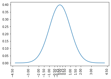
Imagine however the special case that our data is generated from a normal distribution with known parameters, say the mean is 0 and the standard deviation is 1. Then we don’t really need to randomly distribute the items. We can simply create buckets that cover different intervals. We need many short intervals around 0 but the farther away from 0 we go, the larger the intervals should become. Obviously, we will have many values in the interval [0, 0.1) but almost no values larger than 10.
This is the intuition in applying machine learning approaches to hashing. By learning the distribution of the data, we can distribute the items to bins in an optimal way. This is something that data independent-hashing cannot achieve.
In 2017 Google researchers made headlines by claiming they were able to improve upon the best known hashing algorithms [2].
Similarity preserving hashing
Data independent approaches
Different approaches have been designed such that the hash codes preserve similarity between objects for different notions of similarity. Locality-sensitive hashing (LSH) is a family of hashing algorithms that preserve different metrics between objects, such as Euclidean distance or set overlap. Let us consider a concrete example that estimates the angle between vectors.
Let our input data be d-dimensional vectors. We select k random d-dimensional vectors w_i, where each entry is chosen from a standard normal distribution N(0,1).
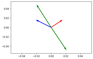
The random vectors are stacked into a matrix W. The hash code is then computed as

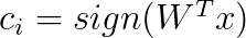
The above says that we compute the inner product of x and each random vector w and take the sign as a hash code. You can think of each d-dimensional random vector as a random hyperplane in the d-dimensional space. The sign shows on each side of the hyperplane the vector x lies. See Figure 2 for an example in 2 dimensions. Therefore, if two vectors have a small angle between them, they are likely to be on the same side of the hyperplane, i.e., they will have a large overlap. The main result for LSH is that

where θ(x, y) denotes the angle between the vectors x and y.
Why bit vectors?
The objective is to create hash codes that consist of individual bits. Bit vectors are very compact and thus even large datasets can be processed in main memory. Also, arithmetic operations on bit vectors are highly efficient. Even similarity exhaustive search on bit vectors can be much more efficient than exhaustive search for vectors with continuous values. The reason is that bit vectors can be loaded and processed in fast CPU cache. Replacing a vector inner product u^T*v for general vectors by a XOR (counting the number of identical bits) on two bit vectors yields thus significant computational advantages.
Unsupervised learning to hash for similarity search
One of the first algorithms that was proposed was based on PCA decomposition. We find the k directions with highest variance in the covariance matrix
Then we use a d-times-k projection matrix W that projects the data X onto the k ≤ d leading eigenvectors, i.e., the eigenvectors corresponding to the k largest eigenvalues:
Observe that it holds:

In the above Λ is a diagonal k-times-k matrix that consists of the largest eigenvalues, and W contains the corresponding eigenvectors.
The hash code is then computed as

An obvious disadvantage is that in this way all directions are treated equally. But we need to pay more attention to directions with higher variance. Researchers have proposed different techniques that assign more bits to directions with larger variance.
Supervised learning to hash for similarity search
This is a setting where we have labeled data. For example, a database of n images tagged with different categories. Here, we can create similarity scores between images and store them in a n-times-n matrix S. For example, the entry S_{i,j} denotes how similar are two images based on their tags, say Jaccard similarity between the two sets of tags. (Of course, similarity is a very general concept and different measures are possible.)
We require the entries S_{i,j} to be values between -1 and 1, thus for a similarity measure sim(i, j) with values in [0,1] we set
The goal is to solve the following optimization problem.

The matrix B contains the hash codes for the n objects. Observe that we multiply the similarity matrix by k because the values in BB^T are between -k and k. In the above, the subscript F denotes the Frobenius norm of a matrix:
The above optimization problem is hard to solve because we request the values in B to be either -1 or 1. The relaxed version is given by

The solution is then converted to bit vectors by taking the sign of each entry in B.
Learning to rank
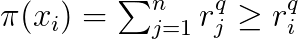
Another widely studied problem is the design of hash codes that can be used to preserve the rank of elements. The setting is as follows. For a query q, there is a list of relevance scores sorted in descending order
The ranking of item i is then given by
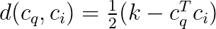
Let us define the distance between two binary vectors with entries from {-1,1}:
Let I be a binary indicator function such that I(E) = 1 if and only if the event E is true. The ranking using the distance function and the binary codes can be written as

The indicator however results in a problem that is hard to optimize. We therefore replace it with a probability expression using the sigmoid function:

In order to learn the binary vectors, we use a matrix with learnable parameters.
However, using the sign function results again in a problem that is hard to optimize. Thus, we drop the sign and obtain the following expression for the probability

This can be then used in the expression for the ranking, namely

Once we have an expression for learning the parameters of the ranking, we can plug it into a loss function like Normalized Discounted Cumulative Gain (NDCG). I refer the reader to [4] for more details.
Discussion
One should always remember that learning hash functions is a machine learning problem. Thus, it comes with the advantages and drawbacks of machine learning. It might lead to superb performance and close to optimal hash codes. But also, obtaining hashing codes might be slow, error-prone, and susceptible to overfitting. It is advisable to use data-independent hash functions with well-understood properties as a baseline when learning hash codes. In fact, advanced data independent hashing approaches like Cuckoo Hashing achieve comparable results to the ones reported in [2].
References
[1]Learning to Hash for Big Data: A Tutorial. Wu-Jun Li. Available at https://cs.nju.edu.cn/lwj/slides/L2H.pdf
[2] The Case for Learned Index Structures. Tim Kraska, Alex Beutel, Ed H. Chi, Jeffrey Dean, Neoklis Polyzotis. Available at https://arxiv.org/pdf/1712.01208.pdf
[3] A Survey on Learning to Hash. Jingdong Wang, Ting Zhang, Jingkuan Song, Nicu Sebe, and Heng Tao Shen. IEEE Transactions On Pattern Analysis and Machine Intelligence (TPAMI) 2017. Available at https://arxiv.org/abs/1606.00185
[4] Ranking Preserving Hashing for Fast Similarity Search. Qifan Wang, Zhiwei Zhang and Luo Si. IJCAI 2015. Available at: https://www.ijcai.org/Proceedings/15/Papers/549.pdf
Learning to hash was originally published in Towards Data Science on Medium, where people are continuing the conversation by highlighting and responding to this story.
from Towards Data Science - Medium https://ift.tt/2Zd1EXd
via RiYo Analytics


No comments