https://ift.tt/3aZEyWO mlforecast makes forecasting with machine learning fast & easy By Nixtla Team . TL;DR : We introduce mlforeca...
mlforecast makes forecasting with machine learning fast & easy
By Nixtla Team.
TL;DR: We introduce mlforecast, an open source framework from Nixtla that makes the use of machine learning models in time series forecasting tasks fast and easy. It allows you to focus on the model and features instead of implementation details. With mlforecast you can make experiments in an esasier way and it has a built-in backtesting functionality to help you find the best performing model.
You can use mlforecast in your own infrastructure or use our fully hosted solution. Just send us a mail to federico@nixtla.io for testing the private beta.
Although this example contains only a single time series it, the framework is able to handle hundreds of thousands of them and is very efficient both time and memory wise.
Introduction
We at Nixlta, are trying to make time series forecasting more accessible to everyone. In this post, we’ll talk about using machine learning models in forecasting tasks. We’ll use an example to show what the main challenges are and then we’ll introduce mlforecast, a framework that facilitates using machine learning models in forecasting. mlforecast does feature engineering and takes care of the updates for you, the user only has to provide a regressor that follows the scikit-learn API (implements fit and predict) and specify the features that she wants to use. These features can be lags, lag-based transformations, and date features. (For further feature creation or an automated forecasting pipeline check nixtla.)
Motivation
For many years classical methods like ARIMA and ETS dominated the forecasting field. One of the reasons was that most of the use cases involved forecasting low-frequency series with monthly, quarterly, or yearly granularity. Furthermore, there weren’t many time-series datasets, so fitting a single model to each one and getting forecasts from them was straightforward.
However, in recent years, the need to forecast bigger datasets higher frequencies has risen. Bigger and higher frequency time series impose a challenge for classical forecasting methods. Those methods aren’t meant to model many time series together, and their implementation is suboptimal and slow (you have to train many models) and besides, there could be some common or shared patterns between the series that could be learned by modeling them together.
To address this problem, there have been various efforts in proposing different methods that can train a single model on many time series. Some fascinating deep learning architectures have been designed that can accurately forecast many time series like ESRNN, DeepAR, NBEATS among others. (Check nixtlats and Replicating ESRNN results for our WIP.)
Traditional machine learning models like gradient boosted trees have been used as well and have shown that they can achieve very good performance as well. However, using these models with lag-based features isn’t very straightforward because you have to update your features in every timestep in order to compute the predictions. Additionally, depending on your forecasting horizon and the lags that you use, at some point you run out of real values of your series to update your features, so you have to do something to fill those gaps. One possible approach is to use your predictions as the values for the series and update your features using them. This is exactly what mlforecast does for you.
Example
In the following section, we’ll show a very simple example with a single series to highlight the difficulties in using machine learning models in forecasting tasks. This will later motivate the use of mlforecast, a library that makes the whole process easier and faster.
Libraries
Data
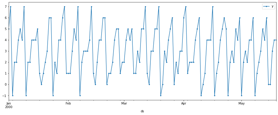
Our data has daily seasonality and as you can see in the creation, it is basically just dayofweek + Uniform({-1, 0, 1}).
Training
Let’s say we want forecasts for the next 14 days, the first step would be deciding which model and features to use, so we’ll create a validation set containing the last 14 days in our data.
As a starting point, we’ll try lag 7 and lag 14.
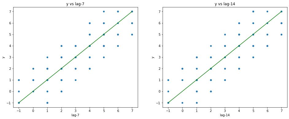
We can see the expected relationship between the lags and the target. For example, when lag-7 is 2, y can be either 0, 1, 2, 3 or 4. This is because every day of the week can have the values [day — 1, day, day + 1], so when we’re at the day of the week number 2, we can get values 1, 2 or 3. However the value 2 can come from day of the week 1, whose minimum is 0, and it can come from the day of week 3, whose maximum is 4.
Computing lag values leaves some rows with nulls.

We’ll drop these before training.
For simplicity sake, we’ll train a linear regression without intercept. Since the best model would be taking the average for each day of the week, we expect to get coefficients that are close to 0.5.

This model is taking 0.51 * lag_7 + 0.45 * lag_14.
Forecasting
Great. We have our trained model. How can we compute the forecast for the next 14 days? Machine learning models a feature matrix X and output the predicted values y. So we need to create the feature matrix X for the next 14 days and give it to our model.
If we want to get the lag-7 for the next day, following the training set, we can just get the value in the 7th position starting from the end. The lag-7 two days after the end of the training set would be the value in the 6th position starting from the end and so on. Similarly for the lag-14.


As you may have noticed we can only get 7 of the lag-7 values from our history and we can get all 14 values for the lag-14. With this information we can only forecast the next 7 days, so we’ll only take the first 7 values of the lag-14.
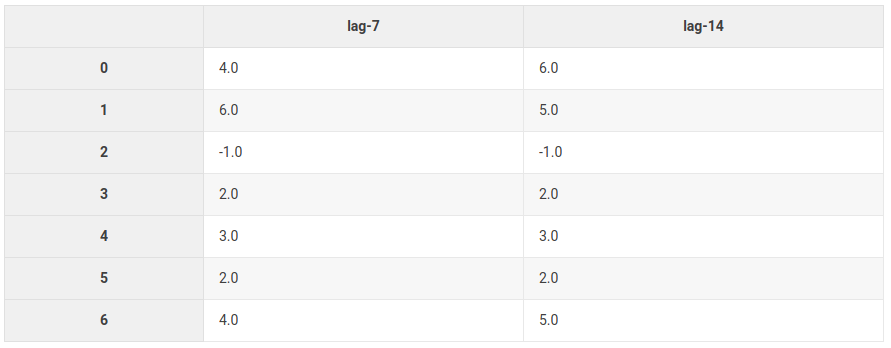
With these features, we can compute the forecasts for the next 7 days.

These values can be interpreted as the values of our series for the next 7 days following the last training date. In order to compute the forecasts following that date, we can use these values as if they were the values of our series and use them as lag-7 for the following periods.
In other words, we can fill the rest of our features matrix with these values and the real values of the lag-14.
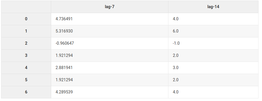
As you can see we’re still using the real values of the lag-14 and we’ve plugged in our predictions as the values for the lag-7. We can now use these features to predict the remaining 7 days.

And now we have our forecasts for the next 14 days! This wasn’t that painful but it wasn’t pretty or easy either. And we just used lags which are the easiest feature we can have.
What if we had used lag-1? We would have needed to do this predict-update step 14 times!
And what if we had more elaborate features like the rolling mean over some lag? As you can imagine it can get quite messy and is very error prone.
mlforecast
With these problems in mind, we created mlforecast, which is a framework to help you forecast time series using machine learning models. It takes care of all these messy details for you. You just need to give it a model and define which features you want to use and let mlforecast do the rest.
mlforecast is available in PyPI (pip install mlforecast) as well as conda-forge (conda install -c conda-forge mlforecast).
The previously described problem can be solved using mlforecast with the following code.
First, we have to set up our data in the required format.
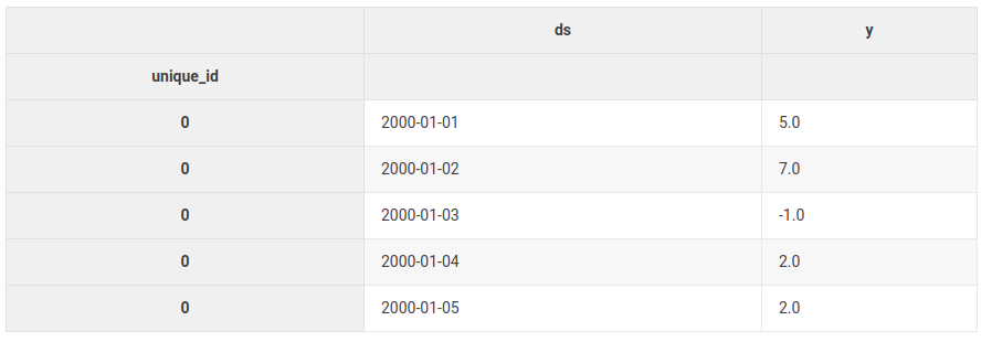
This is the required input format.
- an index named unique_id that identifies each time serie. In this case we only have one but you can have as many as you want.
- a ds column with the dates.
- a y column with the values.
Now we’ll import the TimeSeries transformer, where we define the features that we want to use. We’ll also import the Forecast class, which will hold our transformer and model and will run the forecasting pipeline for us.
We initialize our transformer specifying the lags that we want to use.

As you can see this transformer will use lag-7 and lag-14 as features. Now we define our model.
We create a Forecast object with the model and the time series transformer and fit it to our data.
And now we just call predict with the forecast horizon that we want.
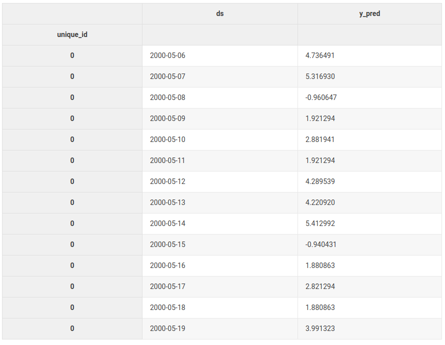
This was a lot easier and internally this did the same as we did before. Let's verify real quick.
Check that we got the same predictions:
Check that we got the same model:
Experiments made easier
Having this high-level abstraction allows us to focus on defining the best features and model instead of worrying about implementation details. For example, we can try out different lags very easily by writing a simple function that leverages mlforecast:


Backtesting
In the previous examples, we manually split our data. The Forecast object also has a backtest method that can do that for us.
We’ll first get all of our data into the required format.
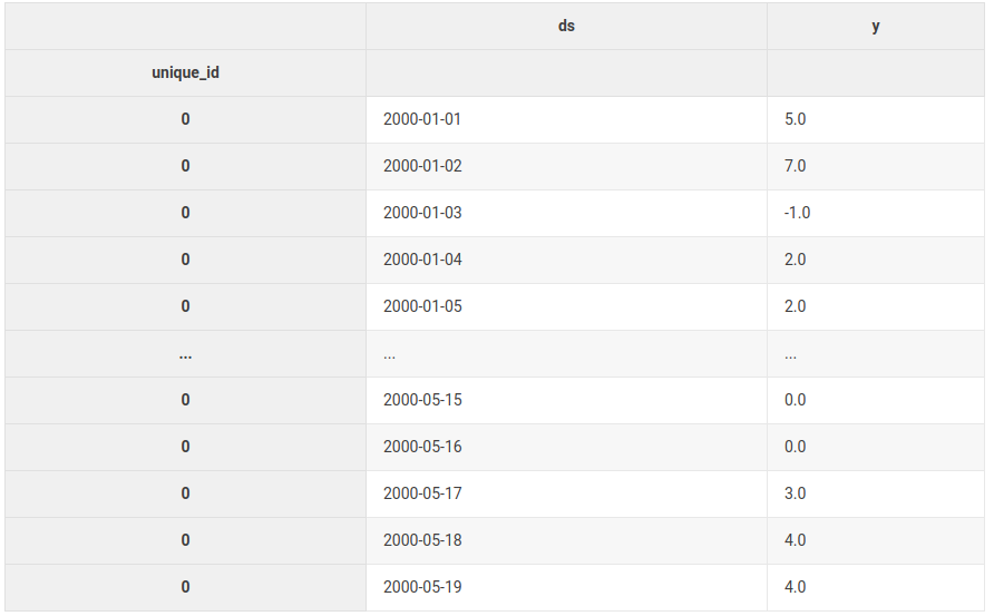
Now we instantiate a Forecast object as we did previously and call the backtest method instead.
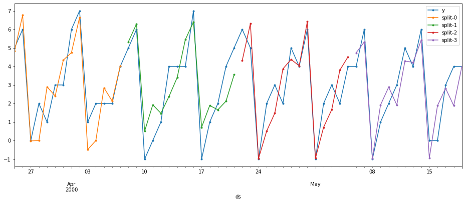
This returns a generator with the results for each window.

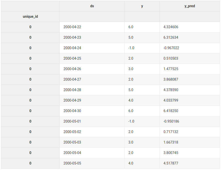
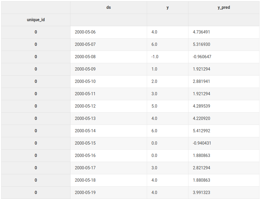
result2 here is the same as the evaluation we did manually.
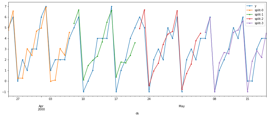
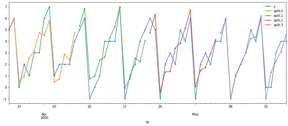
We can define a validation scheme for different lags using several windows.



Lag transformations
We can specify transformations on the lags as well as just lags. The window_ops library has some implementations of different window functions. You can also define your own transformations.
Let’s try a seasonal rolling mean, this takes the average over the last n seasons, in this case, it would be the average of the last n Mondays, Tuesdays, etc. Computing the updates for this feature would probably be a bit annoying, however, using this framework we can just pass it to lag_transforms. If the transformations take additional arguments (additional to the values of the series) we specify a tuple like (transform_function, arg1, arg2), which in this case are season_length and window_size.
help(seasonal_rolling_mean)
Help on CPUDispatcher in module window_ops.rolling:

seasonal_rolling_mean(input_array: numpy.ndarray, season_length: int, window_size: int, min_samples: Union[int, NoneType] = None) -> numpy.ndarray
    Compute the seasonal_rolling_mean over the last non-na window_size samples of the
    input array starting at min_samples.
lag_transforms takes a dictionary where the keys are the lags that we want to apply the transformations to and the values are the transformations themselves.

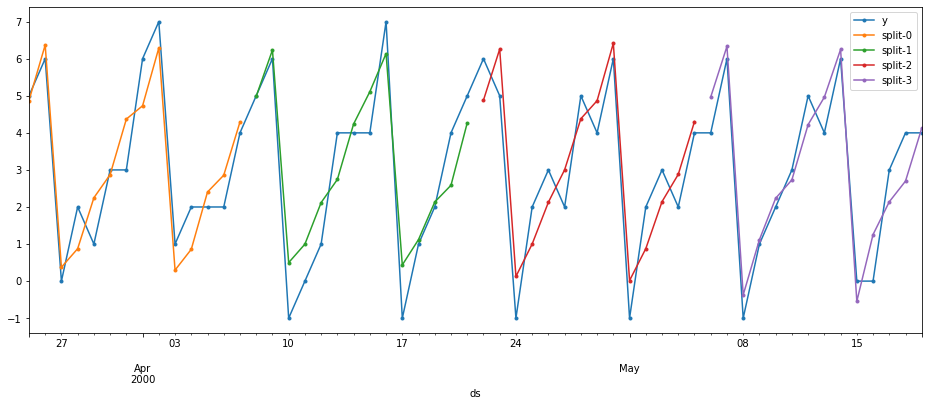
Date features
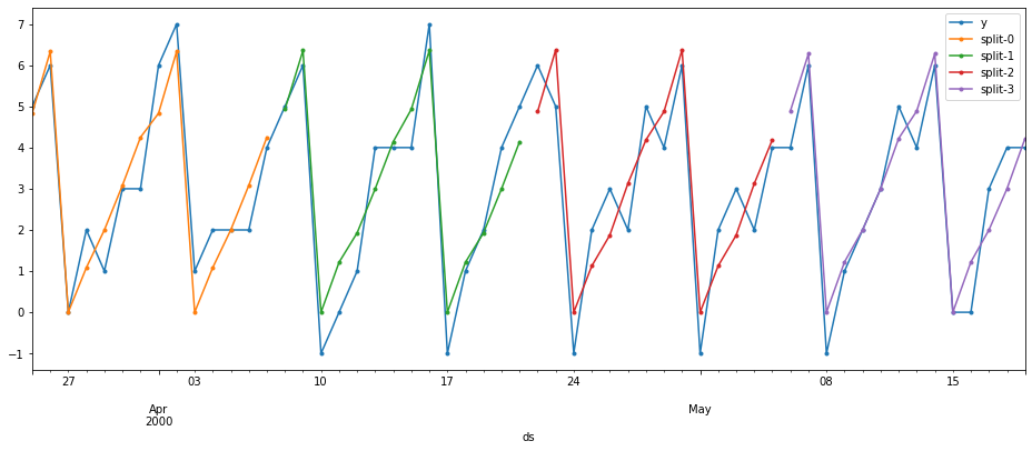
You can also specify date features to be computed, which are attributes of the ds column and are updated in each time step as well. In this example, the best model would be taking the average over each day of the week, which can be accomplished by doing one-hot encoding on the day of the week column and fitting a linear model.

Next steps
mlforecast has more features like distributed training and a CLI. If you’re interested you can learn more in the following resources:
- GitHub repo: https://github.com/Nixtla/mlforecast
- Documentation: https://nixtla.github.io/mlforecast/
- Example using mlforecast in the M5 competition: https://www.kaggle.com/lemuz90/m5-mlforecast
Forecasting with Machine Learning Models was originally published in Towards Data Science on Medium, where people are continuing the conversation by highlighting and responding to this story.
from Towards Data Science - Medium https://ift.tt/3vIIYLh
via RiYo Analytics

ليست هناك تعليقات