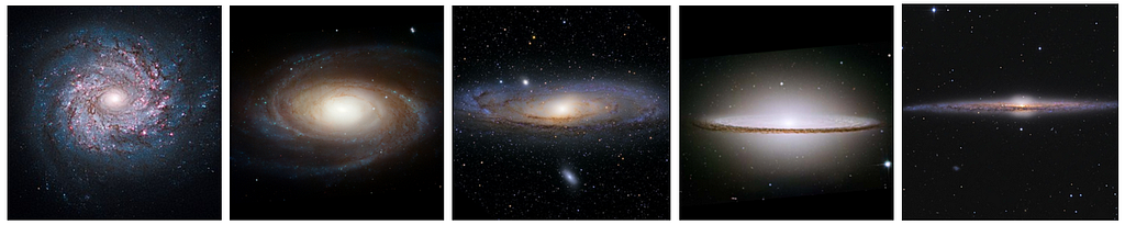
https://ift.tt/3CvDKFc Spiral galaxies sorted from face-on to edge-on. All images are rotated to have the semi-major axes of galaxies alig...
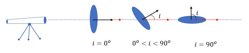
Inclination of disk galaxies plays an important role in their astronomical analyses such as measuring their distances or the attenuation of their light by dust in their halo. As depicted in the diagram below, “Inclination” is the angle between the line-of-sight of the observer and the normal vector of the galaxy disk.
The inclinations of disk galaxies can be roughly derived from the axial ratio of the projected ellipse that defines their boundary. Although this approximation might provide good enough inclination estimates, in ~30% of cases ellipticity-derived inclinations are problematic for a variety of reasons, such as the existence of prominent bulges that dominate the axial ratio measurements. Some galaxies may not be even axially symmetric due to tidal effects.
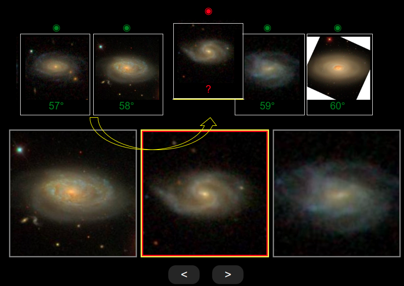
My Ph.D. research involved measuring the spatial inclination of ~20,000 spiral galaxies. I designed an interactive GUI called Galaxy Inclination Zoo (GIZ) to find the inclination of target galaxies by visually comparing each galaxy with a set of standard galaxies with known inclinations. Crowdsourcing this project helped me to obtain at least 3 independent measurements for each galaxy in 9 months.
The outcome of the GIZ project provided me with a large enough sample to investigate the potentials of my favorite Machine Learning algorithms, such as Convolutional Neural Network (CNN), to avoid the similar tedious task in the future. Here, my main goal is to evaluate the inclination of a spiral galaxy from its optical image, whether it is presented in grayscale or colorful formats.
Data
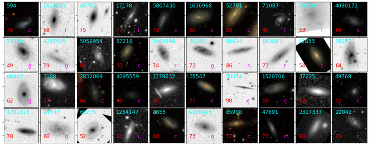
To obtain the cutout image of each galaxy, I downloaded all available calibrated single exposures from the SDSS DR12 database and then I transformed them into full-exposure images in grayscale. In addition, I directly queried the colorful cutouts from the SDSS quick-look image server. Although I provided all images to the GIZ users in 512x512, for this project I downsampled images to 128x128 to build my CNN models. This allows the complexity of models to be manageable with my available computational resources.
The original research required me to only include galaxies with spatial inclinations between 45 to 90 degrees. The label of each galaxy is the average of independent measurements by human users after applying some minor adjustments. I divided users into two groups, and I compared their measurements of similar galaxies to get a better sense of their typical performance. I found that the root mean square of discrepancies between the two groups is ~2.6ᵒ. Any ML model that achieves similar or better accuracy can be potentially adopted for future astronomical research.
Data Augmentation
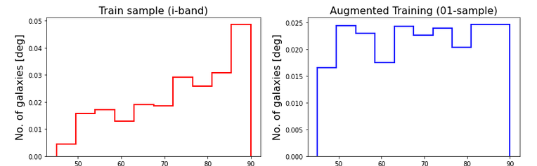
To avoid over-fitting, I increase the sample size by leveraging the augmentation methods. The inclination of each galaxy is independent of its projected position angle on the image and the image quality. Therefore, I generate more images by running the sample through a combination of transformations such as translation, rotation, mirroring, added Gaussian noise, altering contrast, blurring. All of such transformations keep the aspect ratio of images intact to ensure that the elliptical shape of galaxies and their inclinations are preserved. Because my sample is imbalanced, I tune the augmentation rates at different inclination intervals to end up with an almost uniform distribution of labels.
Convolutional Neural Network Models
Exploring different network architecture, I found that the VGG-based models — where convolutional filters are of size 3x3 — are simplest but still powerful in tackling this problem. Other well-known architectures such as ResNET are also appealing. However, they need a lot of computational resources to achieve satisfactory results in this case. Transfer Learning is another avenue, where a few last layers of a pre-trained network are removed and replaced by new layers to accommodate the problem requirements. I found that networks that are trained by huge datasets such as ImageNet are more complicated than what I needed. For my application, even retraining a few last layers of such networks usually takes longer than designing and training a simpler network from scratch. The nature of galaxy images are simpler than a daily life photograph that may contain a lot of objects, shapes and colors.
Due to the lack of enough computational power, I took a try-and-error approach to find satisfactory architectures. To explore many models, I utilized a small fraction of my original data. I investigated three well-behaved CNNs that are slightly different in terms of the number of layers and free parameters.
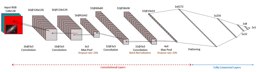
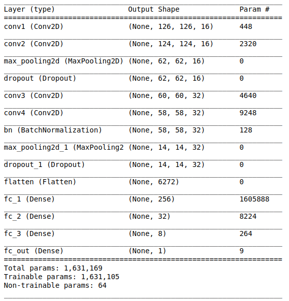
Here, I only present the simplest of the three CNNs I studied. The total number of free parameters of this model is ~1,600,000. It consists of two sets of double convolutional layers that are followed by Maxpooling and Dropout layers. I chose Tanh as the activation function of the last layer, as it outputs numbers between -1 and 1, which is more compatible with the finite range of inclinations in my sample, i.e 45 to 90 degrees.
Here is how I implemented the model in TensorFlow:
The following table shows the model summary:
Training
Prior to the training process, I set aside 10% of the sample for the purpose of testing and model evaluations. I use “Adam” optimizer, and “Mean Squared Error” for the loss function, and I keep track of the Mean Squared Error (MSE) and Mean Absolute Error (MAE) metrics during the training process. I normalize all images by dividing them by 255, and linearly map the inclinations to values ranging between -1 and 1.
I use the Google Colab Pro service for training purposes. With 128x128 images and augmentation, the required memory to open up the entire augmented sample is beyond the capacity of the chosen service. I attempt to resolve the issue by storing the training sample in 50 randomized batches on disk. Each training step begins with loading a random training batch. Then it continues with the reconstruction of the network from the previous step, and advancing the training process for just one epoch. At the end of each step, I store a snapshot of the network for use in the next step. I continue updating the network for as many steps as needed to cover all training batches multiple times.
In the following code, trainer is the function that advances the training process for one epoch and returns the performance metrics.
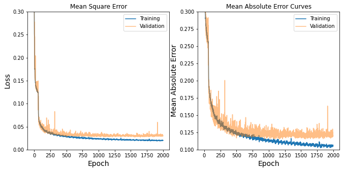
The following figure illustrates the network evaluation metrics for training and testing sets at different training epochs. The training process can be evidently stopped at ~1000 iterations. Nevertheless, my experimentations show that some over-training helps to remove the inclination-dependent biases in predictions. Moreover, overfitting reduces the magnitude of fluctuations in the MSE and MAE metrics.
Here are some of the pros and cons of my training approach:
Pro(s)
- The capability of generating as many training galaxies as needed without being worried about the memory size
- Stopping the training process at any point and continue the process from where it was left. This particularly helps if the execution crashes due to the lack of enough memory, which more likely happens if other irrelevant processes clutter the system
- Monitoring the training process and making decisions as the process goes on
Con(s)
- The training time is dominated by the i/o process, not the time needed to update the network parameters at each epoch
Testing
Now, it is time to use my ~2,000 test galaxies to evaluate the performance of the trained model.
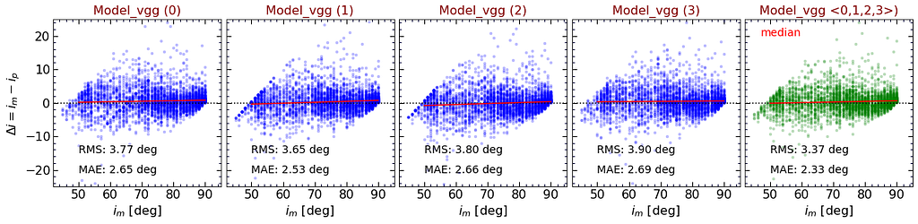
I evaluate the performance of models based on the accuracy of their predictions. The following figure shows the differences between the predicted inclinations and the measured values, i.e. Δi=iₘ-iₚ. Each point represents a galaxy in the test sample. Predicted values, iₚ, are directly generated by applying the trained network on the test sample. The red solid line displays the results of a least square linear fit to the data points.
To improve the final predictions, I train each model multiple times to explore the ability of the Bootstrap Aggregation in improving the results. For simplicity, I label each trained model as Model_vgg (m), where m signifies the “flavor of the model”. m=0 denotes the model trained using the whole training sample, and m≠0 represents models that are trained based on 67% of the data. Each panel displays the results of one model. RMS and MAE denote “Root Mean Square” and “Mean Absolute Error” of the fluctuation of Δi around zero.
As shown, the RMS of the differences are worse than ~3.5ᵒ in all cases. Recall that average human performance based on the same metric is ~2.6ᵒ. In the right-most panel, green points are calculated using the median predictions of all model flavors. As expected, both RMS and MAE metrics of the average model are improved. Hopefully, with enough computational resources and training more models with various architectures, we can reach the human-level accuracy.
Comparison with ellipticity-based inclinations
As a baseline, I derive the inclinations of spiral galaxies from the ellipticity of their projected images. Inclinations are determined from the observed axial ratios, b/a, through

where r is the intrinsic axial ratio of the galaxy if it is viewed edge-on. For our purpose r=0.3 generates more realistic inclinations. Although, this value is not necessarily constant across the entire sample and can be as low as r=0.1. Below, I plot i versus the actual inclinations, iₘ, for the median of predictions by all the CNNs I studied (left) and those I calculated using the ellipticity of the galaxies (right).
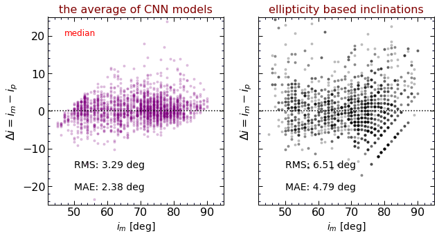
Clearly, CNN models are capable of generating much more reliable inclinations than those crudely derived from the axial ratios.
Web Application and API
I have deployed the best generated models of this project in the form of a web application and a REST API for all future needs.
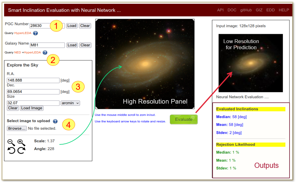
This online GUI allows users to submit a galaxy image through four different methods. Galaxies with SDSS coverage can be queried using their PGC ID (1), common name (2), and equatorial coordinates (3). Users can also upload any galaxy image of their interest (4).
For full documentation on how to use the API, please refer to: https://edd.ifa.hawaii.edu/static/html/tutorial.html#API
Below, I list three different ways that one can use this API. Either enter the URL in the address bar of your favorite Internet browser, or simply use curl or any of your favorite tools to send POST requests to this application. The application returns the evaluated inclinations in JSON format.
$ curl http://edd.ifa.hawaii.edu/inclinet/api/pgc/<pgc_id>
$ curl http://edd.ifa.hawaii.edu/inclinet/api/objname/<galaxy_name>
$ curl -F ‘file=@/path/to/galaxy/image.jpg’ http://edd.ifa.hawaii.edu/inclinet/api/file
Summary
I studied the capability of three CNN models to evaluate the inclination of spiral galaxies from their optical images. All of these models exhibit better accuracy than the ellipticity-based inclinations. I noted that averaging the results across multiple training scenarios and model architectures (bagging method) improve the overall evaluation performances.
I presented the best constructed models online in the form of a web GUI and API.
For further improvements, I recommend using synthetic galaxies with known inclinations from big galaxy simulations, such as Illustris. Data augmentation can also be improved by introducing more complexities which allows networks to gain enough expertise on various instances of galaxies.
If you are interested in more details, my codes and deployment plans are available on my GitHub at https://github.com/ekourkchi/inclinet_project
Data Availability
All inclinations that I used in this article are tabulated in Table 1 of Kourkchi et al. (2020ApJ…902..145K). The complete version of this table is also available in the public domain of the Extragalactic Distance Database (EDD) under the title of “CF4 Initial Candidates”. The underlying galaxy images are publicly accessible through the SDSS imaging database (Data Release 12).
References
- Cosmicflows-4: The Catalog of ~10,000 Tully-Fisher Distances (Kourkchi et al., 2020, ApJ, 902, 145, arXiv:2009.00733)
- Global Attenuation in Spiral Galaxies in Optical and Infrared Bands (Kourkchi et al., 2019, ApJ, 884, 82, arXiv:1909.01572)
- The Extragalactic Distance Database, (Tully, R. B. et al., 2009, AJ, 138, 323)
- Global Extinction in Spiral Galaxies, (Tully et al. 1998, AJ, 115, 2264)
- Galaxy Inclination Zoo (GIZ)
Evaluating the Spatial Inclination of Disk Galaxies with TensorFlow was originally published in Towards Data Science on Medium, where people are continuing the conversation by highlighting and responding to this story.
from Towards Data Science - Medium https://ift.tt/2Zw3KBQ
via RiYo Analytics


No comments