https://ift.tt/3pdwOc5 An experiment to see how both loose and restrictive filters affect vector search speed and quality. This article co...
An experiment to see how both loose and restrictive filters affect vector search speed and quality.
This article contains an experiment of how applying filters to an HNSW-based vector search affects recall and query speed. Using a simple trick, we can achieve high recall and low response times on any kind of filter — without knowing what filters would look like upfront.
Vector search is a hot topic right now and HNSW is one of the top contenders for ANN index models with regards to Recall/Latency trade-offs. If incremental build-up and CRUD operations are important — as is typically the case for vector search engines — HNSW is often considered the best option. In real-life cases, vector searches often need to be filtered. For example, in an e-commerce application, users may wish to find items related to the ones currently in the shopping cart (vector search) but filter them by availability and profit margin (structured search).
HNSW can be tweaked to allow for such structured filtering, but this raises the question of the effects of such filtering on both query speed and recall. Existing benchmarks only measure these trade-offs for unfiltered searches. In this article, we will run a few experiments with filtered vector search using the open-source vector search engine Weaviate which supports these operations out of the box. We will apply filters of varying restrictiveness and compare query speed and recall to unfiltered vector searches.
Post-Filtering vs. Pre-Filtering
Generally, there are two paradigms with regards to filtering vector-search; either the filter is applied after a vector search has already been completed or before. Post-filtering may work well if the filter is not very restrictive, that is when it contains a large portion of the dataset. However, when the filter gets very restrictive, the recall drops dramatically on post-filtering. Imagine a scenario where the filter matches just 5% of the dataset. Now perform a k=20 vector search. Assuming data were evenly distributed, we expect to only contain a single match in our result set, yet the user asked for 20 results.
Post-filtering can lead to very low recall values when the filters become more restricve. Thus, pre-filtering in combination with an efficient vector index is required to achieve great overall recall.
This shows that post-filtering is not a viable option if we want to address filters of all levels of restrictiveness. Instead, we need to apply pre-filtering. Some authors suggest that the term per-filtering implies that an ANN model can no longer be used. However, this is not the definition used in this article. We use the term pre-filtering to mean that an efficient “traditional” index structure, such as an inverted list, can be used to determine the allowed set of candidates. Then this list is passed to the ANN model — in this case, HNSW.
The test setup
For our experiment, we have chosen the following settings:
- Running with Weaviate v1.8.0 which uses a custom HNSW implementation with extended filtering and CRUD support.
- 100 filters in 1% increments of restrictiveness (0% restrictive ->100% of the dataset is contained in the filter, 99% restrictive -> 1% of the dataset is contained in the filter)
- 250k objects with random 256d vectors
- Weaviate’s default HNSW construction settings (efConstruction=128, maxConnections=64)
- 1 Class Shard on 1 Weaviate Server Node
- Ran on a 2014 iMac workstation with a Quad-Core Intel Core i7 CPU
Some of those choices are arbitrary and may have an effect on the outcome. For example, using a more modern CPU would lead to slightly faster query times, but wouldn’t affect the recall. Using a larger dataset would lead to slightly higher query times, etc. They are meant as a starting point that represents many users’ requirements and can be adjusted for other use cases.
Results
Recall
Before looking at the query times in detail, we want to take a look at the recall for filters of varying restrictiveness. The graph below shows a very loose filter on the left side (0% restrictiveness) and a very tight (99% restrictiveness) filter on the right side, as well as various steps in between. The queries have been performed for sizes k=10, k=15, and k=20 which would be typical lengths on search result pages.
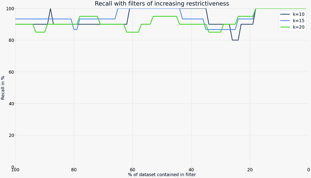
As we can see, the recall does not drop dramatically for either end of the scale. The left edge of the x-axis represents a filter that matches 100% of the data. In other words, it is equivalent to an unfiltered vector search. These recall values act as a baseline for our comparison. As the filter gets more restrictive, the lines sometimes dip below the baseline and sometimes rise above it. But on average, filtering does not seem to negatively affect the recall of a vector search. Interestingly, as filters get more restrictive (less than 20% of the dataset contained) the recall is perfect (100%). Note that this holds true also when disabling the HNSW cutoff — which will be explained below.
Query speed
Knowing that recall is not affected considerably — even when applying very restrictive filters — we can now shift our focus onto query speed. The following shows the query speed for the same filters as above. The speed is composed of three elements:
- Inverted Index
This represents the time it takes to build an allow-list for all candidates. This happens before the list is passed to the HNSW implementation. It uses an inverted list on disk. - HNSW
This represents the time it takes to perform a filtered HNSW search. - Object Retrieval
Since the end-user will receive a full result including all the objects themselves, a small portion of the query time is also spent on retrieving the objects from disk.
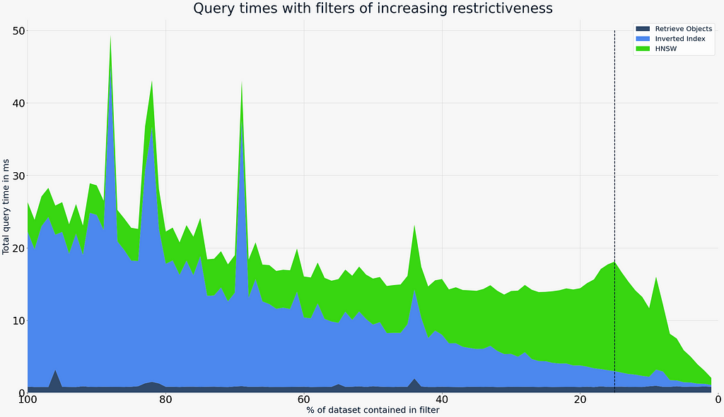
The graphic above highlights the following points:
- Regardless of filter, searches typically don’t take longer than 30ms, with the mean being well below 20ms. Note: There are a few random spikes that are explained by background tasks and/or garbage collection. Note that the experiment was performed on a macOS workstation with various background tasks and not on dedicated hardware.
- The cost of building up an allow-list from disk using the Inverted Index decreases roughly linearly as the filters become more restrictive and therefore the number of potential matches is reduced.
- The HNSW index is most efficient when the search is unfiltered (far-left). As the filters become more restrictive, the cost to search the HNSW index increases slightly, but is typically offset by the reduction in the cost of building up the Inverted Index.
- There is a configurable cut-off highlighted by the vertical dotted line. At this point, Weaviate switches the search mechanism internally. This cut-off is entirely configurable and explained in detail in the next section. In our experiment, it is set to 40,000 objects or 15% of the total dataset size.
Effects of very restrictive filters and introducing a flat-search cutoff
In the previous section, we have highlighted that Weaviate automatically switches the search mechanisms at a specified cut-off. To understand why such a switch is happening, we need to look at how a filtered search is performed with HNSW.
HNSW is a graph-based index model. This means that nodes in the graph are placed so that similar objects are positioned nearby. Each node has a set of edges to neighboring nodes. To avoid the graph becoming too massive, HNSW limits the number of edges in two ways; there is a fixed limit for the number of edges and a heuristic to determine the most valuable connections. When it is time to prune the connections because they have grown too large, HNSW will remove those elements that are closer to an existing neighbor than to the node itself. For example, in the very simple graph, A--B--C there is no need to connect A to C, because C can already be reached efficiently with just just one additional hop (via B) from A. This is known as the Small World Phenomenon which represents the “SW” in HNSW.
At search time, HNSW always starts with a specific entry point and evaluates its neighboring connections. The ones closest to the specified query vector are added as candidates. The number of candidates held at any point is controlled by the query-time ef parameter. If adding new candidates no longer improves the worst distance in the set of candidates, the search is complete. This is what makes HNSW an approximate index and makes it considerably faster than brute force. In addition, the graph consists of multiple layers (“Hierarchical” for the “H” in HNSW). This allows to efficiently move in the correct direction of the graph on higher layers where fewer points are contained and edges are considerably longer.
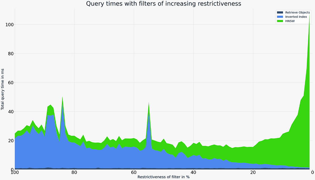
When a search is filtered, candidates which aren’t present on the allow list, will not be added to the result set. This means that as filters become very restrictive (85% and up), the HNSW search will find more and more candidates which are viable from a distance perspective, yet excluded by the filter. If we remove the cutoff point from the search shown above, we can see that query times rise sharply as we move to the right edge (very restrictive filters).
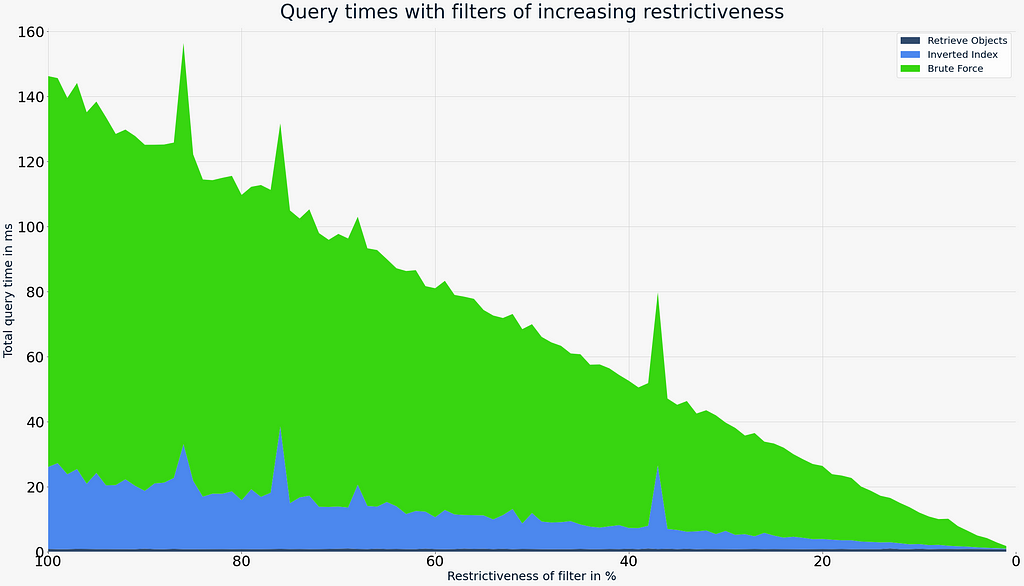
However, since Weaviate also features an Inverted Index and the candidates were determined before starting the vector search, we can now make use of this small number of data points. A flat search (brute force) has a cost that is linear to the size of the dataset. The graph on the side shows that a flat search follows the opposite pattern of the HNSW search. As we make the filter more restrictive, the query times decrease. To demonstrate the cost of a brute-force as a function of filter restrictiveness, we have set the cutoff in Weaviate to 250k, meaning that effectively for every filtered vector search the HNSW index was skipped.
This clearly shows that flat search query times are considerably worse for most cases. However, in those cases where HNSW struggles is where a flat search shines. So, a simple cut-off point to switch from one to the other allows for a very efficient search over any level of restrictiveness.
Conclusions
This experiment has shown that when using Weaviate’s hybrid approach of using the HNSW index for most filtered searches, but switching to a flat search on extremely restricted searches, we can achieve great recall and query times on any filter.
The recall is roughly constant over the entire set of filters and at a level comparable to an unfiltered control search. Query times in the experiment were always below 30ms and the mean query time well below 20ms which should be fast enough for even the most latency-critical of use cases.
To learn more about Weaviate, you can browse the documentation.
Effects of filtered HNSW searches on Recall and Latency was originally published in Towards Data Science on Medium, where people are continuing the conversation by highlighting and responding to this story.
from Towards Data Science - Medium https://ift.tt/3DYkeSl
via RiYo Analytics


No comments