https://ift.tt/3ngnOQQ Big Data Implementation with Beam How to implement Data Pipelines with the help of Beam Source Apache Beam is ...
Big Data Implementation with Beam
How to implement Data Pipelines with the help of Beam

Apache Beam is one of the latest projects from Apache, a consolidated programming model for expressing efficient data processing pipelines as highlighted on Beam’s main website [1]. Throughout this article, we will provide a deeper look into this specific data processing model and explore its data pipeline structures and how to process them. In addition, we will also example.
What is Apache Beam
Apache Beam can be expressed as a programming model for distributed data processing [1]. It has only one API to process these two types of data of Datasets and DataFrames. While you are building a Beam pipeline, you are not concerned about the kind of pipeline you are building, whether you are making a batch pipeline or a streaming pipeline.
For its portable side, the name suggests it can be adjustable to all. In Beam context, it means to develop your code and run it anywhere.
Installation
To use Apache Beam with Python, we initially need to install the Apache Beam Python package and then import it to the Google Colab environment as described on its webpage [2].
! pip   install apache-beam[interactive]
import   apache_beam as beam
What is Pipeline
A Pipeline encapsulates the information handling task by changing the input.
The Architecture of Apache Beam
In this section, the architecture of the Apache Beam model, its various components, and their roles will be presented. Primarily, the Beam notions for consolidated processing, which are the core of Apache Beam. The Beam SDKs are the languages in which the user can create a pipeline. Users can choose their favorite and comfortable SDK. As the community is growing, new SDKs are getting integrated [3].
Once the pipeline is defined in any supported languages, it will be converted into a generic language standard. This conversion is done internally by a set of runner APIs.
I would like to mention that this generic format is not fully language generic, but we can say a partial one. This conversion only generalizes the basic things that are the core transforms and are common to all as a map function, groupBy, and filter.
For each SDK, there is a corresponding SDK worker whose task is to understand the language-specific things and resolve them. These workers provide a consistent environment to execute the code.
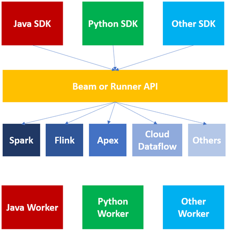
For each language SDK, we have a specific SDK worker. So now it does not matter which runner we are using if we have this Runner or Beam API and language-specific SDK workers. Any runner can execute the same code as mentioned on its guide page [4].
Features of Apache Beam
Apache Beam comprises four basic features:
- Pipeline
- PCollection
- PTransform
- Runner
Pipeline is responsible for reading, processing, and saving the data. This whole cycle is a pipeline starting from the input until its entire circle to output. Every Beam program is capable of generating a Pipeline.
The second feature of Beam is a Runner. It determines where this pipeline will operate [5].
The third feature of Beam is PCollection. It is equivalent to RDD or DataFrames in Spark. The pipeline creates a PCollection by reading data from a data source, and after that, more PCollections keep on developing as PTransforms are applied to it [6].
Each PTransform on PCollection results in a new PCollection making it immutable. Once constructed, you will not be able to configure individual items in a PCollection. A transformation onPCollection will result in a new PCollection. The features in a PCollection can be of any type, but all must be of the same kind. However, to maintain disseminated processing, Beam encodes each element as a byte string so that Beam can pass around items to distributed workers as mentioned in its programming page [6].
The Beam SDK packages also serve as an encoding mechanism for used types with support for custom encodings. In addition, PCollection does not support grained operations. For this reason, we cannot apply transformations on some specific items in a PCollection. We use all the conversions to apply to the whole of the PCollection and not some aspects [6].
Commonly, the source often assigns a timestamp to each new element when the item was read or added. If PCollectionholds bounded data, we may highlight that every feature will be set to the same timestamp. You can specify the timestamp explicitly, or Beam will provide its own. In any of the cases, we can manually assign timestamps to the elements if the source does not do it for us.
The fourth feature of Beam is PTransform. It takes a samplePCollection as the data source and produces an identical PCollection with timestamps attached. They operate in parallel while conducting operations like windowing, assigning watermarks, etc.
Pipeline Structure of Beam
In this section, we will be implementing the pipeline structure of Beam using Python. The first step starts with `assigning pipeline a name`, a mandatory line of code.
pipeline1 = beam.Pipeline()
The second step is to `create` initial PCollection by reading any file, stream, or database.
dept_count = (
 pipeline1
 |beam.io.ReadFromText(‘/content/input_data.txt’)
 )
The third step is to `apply` PTransforms according to your use case. We can use several transforms in this pipeline, and each of the transforms is applied by a pipe operator.
dept_count = (
 pipeline1
 |beam.io.ReadFromText(‘/content/input_data.txt’)
 |beam.Map(lambda line: line.split(‘,’))
 |beam.Filter(lambda line: line[3] == ‘Backend’)
 |beam.Map(lambda line: (line[1], 1))
 |beam.CombinePerKey(sum)
 )
To request a transform operation, you need to implement it to the input PCollection. For every transform, there exists a nonproprietary apply method. We can use the apply operation either with `.apply` or a ` | ` pipe operator.
After all transforms, the fourth step is to write the final PCollection to an external source. It can be a file, database, or stream.
dept_count = (
 pipeline1
 |beam.io.ReadFromText(‘/content/input_data.txt’)
 |beam.Map(lambda line: line.split(‘,’))
 |beam.Filter(lambda line: line[3] == ‘Backend’)
 |beam.Map(lambda line: (line[1], 1))
 |beam.CombinePerKey(sum)
 |beam.io.WriteToText(‘/content/output_data.txt’)
 )
The final step is to run the pipeline.
pipeline1.run()
Generation of Transform Operation with Python
Transformation is an essential element of every data processing structure. Apache Beam contains built-in transformations that can be easily applied with enclosed forms as described in Beam’s main programming documentation [6]. Let’s introduce those transformations in the upcoming sections.
Read from Text
Beam supports `read` and `write` operations from several file formats like text, Avro, Parquet. The first transform is `ReadFromText`. This format parses a text file as newline delimited elements, which means that every line in the file will be treated as a single element by default. `ReadFromText` has a total of six parameters to be edited if you wish to have complete control while reading a file as listed on Beam’s package module page [7]. Let’s look at each of these parameters.
import apache_beam as beam
 reading = beam.Pipeline()

 content_read = (
 reading
 |beam.io.ReadFromText(‘/content/input_data.txt’)
 |beam.io.WriteToText(‘/content/output_data.txt’)
 )

 reading.run()
The first is file_pattern. It specifies the full path of the input file. We can set it with a * operator while reading multiple files from a directory. This path means it will read all the files which start with the input keyword.
The second parameter is minimum_bundle_size. This parameter specifies the min size of bundles that should be generated when splitting the source into bundles. A PCollection is divided into many batches internally, known as bundles [8]. They process parallelly on different machines. The value of this parameter decides what the minimum bundle size of your PCollection should be, and its parameter should be an integer value.
The third parameter is compression_type. It handles compressed input files in case the input file is compressed. We do not provide as Beam will use the provided file path’s extension to detect the type of compression of the input file. For example, if we have a .gzip file, then the input path will detect the compression type from this path. However, if you wish to handle the compressed input files yourself, you can explicitly provide the compression type.
The fourth parameter is strip_trialing_newlines, a Boolean field. It indicates whether the source should remove the newline character. If set to `True`, then the end line is removed and not read. If set to `False`, the end line is not drawn and is read as an empty line. By default, its value is `True.
The fifth parameter is validate. It is also a Boolean flag that confirms if the files exist during the pipeline creation period. If set to `True`, it will control whether the input file is present or not. If the pipeline is not created, then Beam will throw an error. If set to `False`, Beam does not check the file’s existence and generates the pipeline. In this case, you will see the empty output file. It is recommended to set this parameter to `True`. For this reason, its default value is `True`.
The last parameter is skip_header_lines. It helps handle files that are loaded with headers. We do not wish to process the titles, so we can skip reading them using this parameter. You may provide the number of lines you want to ignore in the input file.
Read from Avro
This operation is used to read one or a set of Avro files. It has four parameters. The first three parameters of ReadFromAvro share the same ones as ReadFromText. Its fourth and different parameter is `use_fastavro`. This parameter accepts a Boolean value to read data from the Avro files [7]. Since this parameter is mandatory, ReadFromAvro shall set it to `True` to use this library.
import apache_beam as beam
import avro.schema
from avro.datafile import DataFileReader, DataFileWriter
from avro.io import DatumReader, DatumWriter

from apache_beam.io import ReadFromAvro
from apache_beam.io import WriteToAvro

schema = avro.schema.parse(open(“parquet_file.parqet”, “rb”).read())

parquet_write = beam.Pipeline()
 content_4 = ( parquet_write
 |beam.Create({‘dict1’:[24,45,68],’dict2':[32,54,75]})
 |beam.Map(lambda element: element)
 |beam.io.WriteToAvro(‘/content/output.avro’,schema=schema))

parquet_write.run()
Read from Parquet
The third input transform is ReadFromParquet. This operation benefited from reading parquet files. The first three parameters are the same arguments with ReadFromText and the fourth one is `columns`. This parameter specifies the list of columns that ReadFromParquet will read from the input file [8].
import apache_beam as beam
import pandas as pd
import pyarrow
from apache_beam.options.pipeline_options import PipelineOptions


parquet_data = pd.read_parquet(‘/content/parquet_data.parquet’, engine=’pyarrow’)
parquet_schema = pyarrow.schema([])

schema_map = {
 ‘STRING’: pyarrow.string(),
 ‘FLOAT’: pyarrow.float64(),
 ‘STRING’: pyarrow.string(),
 ‘DATE’: pyarrow.date64()
}

for item in parquet_data.schema:
parquet_schema = parquet_schema.append(pyarrow.field(item.name, schema_map[item.field_type]))

parquet_write = beam.Pipeline()
content = ( parquet_write |beam.beam.io.ReadFromParquet(‘/content/parquet_data.parquet’)
|beam.io.parquetio.WriteToParquet(‘/content/output5.parquet’,schema=parquet_schema))

parquet_write.run()
Read from TFRecord
After Parquet, the last file I/O is ReadFromTFRecord. This operation reads TensorFlow records. TFRecord format is a simple format for storing a sequence of binary forms. These records become famous since they are serialized and therefore faster to stream over the network. This format can also help catch any data-preprocessing. To read TensorFlow records, we have ReadFromTFRecord[9]. It has a list of four parameters.
Three of its parameters are the same as of previous types. Other parameters include `coder` that specifies the `coder` name used to decode each TFRecord.
So, these were various file-based read transforms.
import apache_beam as beam
from apache_beam.io.tfrecordio import ReadFromTFRecord
from apache_beam import coders

reading_tf = beam.Pipeline()
data_path = ‘/content/input_data’

content_read = (
reading_tf
|beam.io.ReadFromTFRecord(data_path, coder=beam.coders.BytesCoder(),
compression_type=’auto’, validate=True) |beam.io.WriteToText(‘/content/output_tfrecord.txt’)
 )
reading_tf.run()
Read from PubSub
The next topic is to read from message queues. Beam overall supports Apache Kafka, Amazon Kinesis, JMS, MQTT, and Google Cloud PubSub. Java supports each of these; however, Python only supports Google Cloud PubSub. We have ReadFromPubSub a transform operation for it. It has a list of some five parameters as below.
import apache_beam as beam
from apache_beam.options.pipeline_options import PipelineOptions
import os
from apache_beam import window
project = 'SubscribeBeam'
pubsub_topic = 'projects/qwiklabs-gcp-01-7779ab5fa77e/topics/BeamTopic'
path = "C:\\Users\ersoyp\qwiklabs-gcp-01-7779ab5fa77e-2d40f7ded2a8.json"
os.environ["GOOGLE_APPLICATION_CREDENTIALS"]=path

input_file = "C:\\Users\ersoyp\data.csv"
output_file = "C:\\Users\ersoyp\output.csv"
options = PipelineOptions()
options.view_as(StandardOptions).streaming = True
process = beam.Pipeline(options=options)
output_file = '/content/outputs/'
pubsub_data = ( process
                | 'Read from PubSub' >> beam.io.ReadFromPubSub(subscription= input_file)
                | 'Write to PubSub' >> beam.io.WriteToPubSub(output_file)
              )
final_file = process.run()
The first parameter is topic. For this parameter, we must provide the topic name. Then we specify the messages that are getting published which Beam will read from them as described in the DataFlow documentation [9].
The second parameter is subscription. The existing pub-sub subscription is attached to a particular topic. The above two parameters are contradictory to each other. In this case, we provide a topic as an argument.
The third parameter is id_label. It specifies which attribute of incoming PubSub messages should be considered as a record identifier as specified in Beam’s module page [10]. When set, the value of that attribute will be used for the deduplication of messages. Otherwise, if not provided, Beam would not guarantee any uniqueness of data.
The fourth parameter is with_attributes. It is a Boolean field. If it is set to `True`, then the output elements will be of type objects. If set to `False`, output elements will be of bytes type. By default, this parameter is set to `False`[10].
The last parameter is timestamp_attribute. As every element in Beam has a timestamp attached to it. This parameter was read from PubSub transform to extract messages from Google Cloud PubSub [10].
Create Transform
To generate our data, Beam supports a create transform operation for it. We can generate varied forms of data like a list, set, dictionary, etc. The create transform will show a few states of the `create transform` operation below with examples. We will simply generate data using create and write it in an output file.
For generating a list of elements, use `beam.Create` then square brackets, and inside it, you may specify your items separated by a comma. In the following example, we have not applied any transformation to the generated data.
import apache_beam as beam
create_transform = beam.Pipeline()
content = (create_transform
            |beam.Create(['Beam create transform'])
            |beam.io.WriteToText('/content/outCreate1.txt')
          )
create_transform.run()
As a second example, a list can be created. For this reason, we generate a list of numbers. The pipeline run should be at the very start of the line, with no spaces before it. The same is the case while we create a pipeline or expected indent. It is indent-free.
import apache_beam as beam

create_transform_2 = beam.Pipeline()

content_2 = (create_transform_2
            |beam.Create([10,22,38,47,51,63,78])
            |beam.io.WriteToText('/content/output2.txt')
           )
create_transform_2.run()
If you want two or more columns’ data, then pass a list of tuples. It is a key-value tuple. Each element behaves as a single column if you further apply a map transform in the tuple.
import apache_beam as beam

create_transform_3 = beam.Pipeline()

content_3 = (create_transform_3
 |beam.Create([(“DataScience”,10), (“DataEngineering”,20),(“ArtificialIntelligence”,30), (“BigData”,40)])
 |beam.io.WriteToText(‘/content/output3.txt’)
)
create_transform_3.run()
For the dictionary, you can pass key-value pairs. For key-value couples, you pass them in curly braces. You can play with round, square, and curly braces to generate varied forms of data. Use different combinations of these braces, and you will get additional data. It creates a transformation with the help of `beam.Create` operation.
import apache_beam as beam

create_transform_4 = beam.Pipeline()
content_3 = ( create_transform_4
       |beam.Create({'dict1':[24,45,68],'dict2':[32,54,75]})
       |beam.Map(lambda element: element)
       |beam.io.WriteToText('/content/output4.txt'))

create_transform_4.run()
Write To Text
WriteToTextwrites each element of the PCollection as a single line in the output file.
The first parameter is the file_path_prefix. It specifies the file path to write the PCollection. If we define this as an argument, then Beam will generate either files or the items in the data directory [11].
beam.io.WriteToText(‘/content/output.txt’)
The num_shardsand file_path_suffix are the second and third parameters. The full name of our file is shown below.
<prefix><num_shards><suffix>
content-0000-of-0001-departments
The first part, `content` is a prefix. The second `0000-of-0001` belongs to the `number_of_shards`. This parameter specifies the number of shards or the number of files written as output. If we set the `number_of_shards` argument as 3, our resulting file will be in 3 pieces. When we do not set this argument, the service will decide on the optimal shards.
In the example, the `department` represents the suffix controlled by the parameter called `file_name_suffix`.
The fourth parameter is append_trailing_newlines. This parameter accepts a boolean value, indicating whether the output file should write a newline character after writing each element. i.e. whether the output file should be delimited with a newline or not. By default, it is set to `True` [12].
The fifth parameter is coder. It specifies the `coder name used to encode each line.
The sixth parameter is compression_type, a string value. This parameter is used to handle compressed output files.
The seventh parameter is header. It specifies a string to write at the beginning of the output file as a header.
Write to Avro
The parameters ofWriteToAvro include the file_path_prefix, file_path_suffix , num_shards, compression_type as just explained for WriteToText.
import apache_beam as beam
from avro import schema
import avro
from apache_beam.io import ReadFromAvro
from apache_beam.io import WriteToAvro

schema = avro.schema.parse(open("avro_file.avsc", "rb").read())

create_transform_5 = beam.Pipeline()
content_4 = ( create_transform_5
|beam.Create(['Beam create transform'])
|beam.Map(lambda element:   element)  |beam.io.WriteToAvro('/content/output5.avro',schema=schema))
create_transform_5.run()
The fifth parameter for WriteToAvro is schema. Writing an Avro file requires a schema to be specified.
The sixth parameter is codec. It is the compression codec to use for block-level compression.
The seventh parameter is use_fastavro which is set to `True`. You may use the `fastavro library` for faster writing [13].
The last parameter is mime_type. It passes the MIME type for the produced output files if the filesystem supports specified MIME types.
Write to Parquet
It is used to write each element of the PCollection to the Parquet file. The parameters of file_path_prefix, file_path_suffix , num_shards, codec , mime_type and schema are the same as with WriteToAvro.
import apache_beam as beam
import pandas as pd
import pyarrow
from apache_beam.options.pipeline_options import PipelineOptions

parquet_data = pd.read_parquet(‘/content/parquet_data.parquet’, engine=’pyarrow’)
parquet_schema = pyarrow.schema([])

schema_map = {
 ‘STRING’: pyarrow.string(),
 ‘FLOAT’: pyarrow.float64(),
 ‘STRING’: pyarrow.string(),
 ‘DATE’: pyarrow.date64()
 }

for item in parquet_data.schema:
parquet_schema =
parquet_schema.append(pyarrow.field(item.name, schema_map[item.field_type]))

parquet_write = beam.Pipeline()
content = ( parquet_write
|beam.beam.io.ReadFromParquet(‘/content/parquet_data.parquet’) |beam.io.parquetio.WriteToParquet(‘/content/output.parquet’,
schema=parquet_schema))

parquet_write.run()
The seventh parameter is row_group_buffer_size. It specifies the byte size of the row group buffer. The row group can be accepted as a segment of a parquet file that keeps serialized arrays of column inputs. It is an advanced feature used for performance tuning of parquet files.
The eighth parameter is record_batch_size. It specifies the number of records for every record_batch. The record batch can be defined as a basic unit used for storing data in the row group buffer. This parameter is purely related to the Parquet file.
Write to TFRecord
It has file_path_prefix, file_path_suffix , num_shards, compression_type parameters which are explained already in the above write operations.
import apache_beam as beam
from apache_beam import Create
from apache_beam import coders
from apache_beam.io.filesystem import CompressionTypes
from apache_beam.io.tfrecordio import ReadFromTFRecord
from apache_beam.io.tfrecordio import WriteToTFRecord

reading_tf = beam.Pipeline()
data_path = ‘/content/input_data’

content_read = (reading_tf
|beam.io.ReadFromTFRecord(data_path, coder=beam.coders.BytesCoder(), compression_type=’auto’, validate=True)
|beam.io.WriteToTFRecord(data_path, compression_type=CompressionTypes.GZIP, file_name_suffix=’.gz’)
)

reading_tf.run()
Write to PubSub
This operation writes PCollection as a messaging stream to Google Cloud PubSub service.
import os
import apache_beam as beam
from apache_beam import window
from apache_beam.options.pipeline_options import PipelineOptions
project = ‘SubscribeBeam’
pubsub_topic = ‘projects/qwiklabs-gcp-01–7779ab5fa77e/topics/BeamTopic’
path = “C:\\Users\ersoyp\qwiklabs-gcp-01–7779ab5fa77e-2d40f7ded2a8.json”
os.environ[“GOOGLE_APPLICATION_CREDENTIALS”]=path
input_file = “C:\\Users\ersoyp\data.csv”
output_file = “C:\\Users\ersoyp\output.csv”
options = PipelineOptions()
options.view_as(StandardOptions).streaming = True
process = beam.Pipeline(options=options)
output_file = “/content/outputs/”
pubsub_data = ( process
 | ‘Read from PubSub’ >> beam.io.ReadFromPubSub(subscription= input_file)
 | ‘Write to PubSub’ ‘ >> beam.io.WriteToPubSub(output_file)
 )
final_file = process.run()
The first parameter is topic. It is used as a location where the output will be written.
The second parameter is with_attributes, which decides the type of input elements. If it is set to `True` then input elements will be of type objects. If `False`, then the format of the feature is bytes.
The third parameter is id_label. It sets an attribute for each Cloud PubSub message with the given name and novel content. It can apply this attribute inReadFromPubSub withPTransform to deduplicate messages [14].
The fourth parameter is timestamp_attribute. It is used as an attribute for each Cloud PubSub message with the given name and its publish time as the value as served in Beam’s module page [15].
Map Transform
Maptransform exerts one element as input and one element as output. It practices a one-to-one mapping function over each item in the collection. The example should take the whole string as a single input, split it based on a comma, and return a list of elements.
import apache_beam as beam

map_transform = beam.Pipeline()

content = ( map_transform
 |beam.io.ReadFromText(([‘data.txt’]))
 |beam.Map(lambda element: element)
 |beam.io.WriteToText(‘/content/output_1.txt’)
 )

map_transform.run()
FlatMap Transform
Functionality-wise FlatMap is almost the same as Map but with one significant difference. While Map can output only one element for a single input, FlatMap can emit multiple elements for a single component. The following example is generating a single list as output.
import apache_beam as beam

flatMap_transform = beam.Pipeline()

 content = ( flatMap_transform
 |beam.io.ReadFromText(([‘data.txt’]))
 |beam.FlatMap(lambda element: element)
 |beam.io.WriteToText(‘/content/output_1.txt’)
)

 flatMap_transform.run()
Filter Transform
The filter operation will filter the elements of the specified department. This filtering function will take the previous list as input and return all the required features in the matching condition.
import apache_beam as beam
filtering = beam.Pipeline()

dept_count = (
 filtering
 |beam.io.ReadFromText(‘/content/input_data.txt’)
 |beam.Map(lambda line: line.split(‘,’))
 |beam.Filter(lambda line: line[3] == ‘Backend’)
 |beam.Map(lambda line: (line[1], 1))
 |beam.io.WriteToText(‘/content/output_data.txt’)
 |beam.CombinePerKey(sum)
 )
 filtering.run()
Pipeline Branch Operations
Most of the pipelines simply represent a linear flow of operations with one-to-one mapping. After the first PCollection, one filter operation produces one new PCollection. On that PCollection one map transform to create additional PCollection in the queue until it is written to a file.
However, for most of the use cases, your pipeline can be significantly complex and branched. This type of pipeline is called branched pipeline in Beam, where we can use the same PCollection as input for multiple transforms.
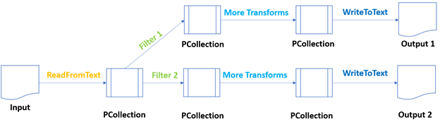
Here is an implemented example flow of a branched structure of a pipeline.
import apache_beam as beam
branched = beam.Pipeline()
input_collection = (
branched
 | “Read from text file” >> beam.io.ReadFromText(‘data.txt’)
 | “Split rows” >> beam.Map(lambda line: line.split(‘,’)))

 backend_dept = (input_collection
 | ‘Retrieve Backend employees’ >> beam.Filter(lambda record: record[3] == ‘Backend’)
 | ‘Pair them 1–1 for Backend’ >> beam.Map(lambda record: (“Backend, “ +record[1], 1))
 | ‘Aggregation Operations: Grouping & Summing1’ >> beam.CombinePerKey(sum))
 ai_dept = ( input_collection
 |’Retrieve AI employees’ >> beam.Filter(lambda record: record[3] == ‘AI’)
 |’Pair them 1–1 for HR’ >> beam.Map(lambda record: (“AI, “ +record[1], 1))
 |’Aggregation Operations: Grouping & Summing2' >> beam.CombinePerKey(sum))
output =(
 (backend_dept , ai_dept)
 | beam.Flatten()
 | beam.io.WriteToText(‘/content/branched.txt’)
 )
branched.run()
In the example above, the first transform operation applies a filter on the Backend department, and Transform B filters all the employees in the AI department.
Generation of ParDo Transform Operation with Python
ParDo can be accepted as a transformation mechanism for parallel processing [16].
The first one is Filtering, a data set. You can use ParDo to take each element in a PCollection and either output that element to a new collection or discard it as provided in the programming guide of Beam [16].
The second one is the Formattingor Type Convertingof each element in a data set. ParDo can be used to make a conversion on each component on the input PCollection [17].
The third one is Extracting Individual Parts from each item. If there exists a PCollection of elements with multiple fields, you may use ParDoor extract individual items.
The fourth one is to perform Computationson each item of PCollection. We can apply this function to every aspect of the PCollection.
Also, we can leverage ParDo for slicing a PCollection in varied ways. In the script below, we used Map, FlatMap, and Filter transforms. When you apply a ParDo transform, you will need to provide user code in the form of a DoFn object.
Internally Mapand FlatMap also, inherit the DoFn class. To implement ParDo in the code, replace the Map and with ParDo. `DoFn` class has many functions in it, out of which we have to override just one part, which is a process function.
import apache_beam as beam
 class EditingRows(beam.DoFn):

def process(self, element):
 return [element.split(‘,’)]

class Filtering(beam.DoFn):

def process(self, element):
 if element[3] == ‘Finance’:
 return [element]

class Matching(beam.DoFn):

def process(self, element):
 return [(element[3]+”,”+element[1], 1)]

class Summing(beam.DoFn):

def process(self, element):
 (key, values) = element
 return [(key, sum(values))]

pardo = beam.Pipeline()
 department_operations= (pardo
 |beam.io.ReadFromText(‘data.txt’)
 |beam.ParDo(EditingRows())
 |beam.ParDo(Filtering())
 |beam.ParDo(Matching())
 |’Grouping’ >> beam.GroupByKey()
 |’Summing’ >> beam.ParDo(Summing())
 |beam.io.WriteToText(‘data/output_pardo.txt’) )
 pardo.run()
Generation of Composite Transform Operation
CompositeTransformas the name suggests is a transform that internally has a series of built-in transformations.
Using composite transforms in your pipeline can make your code more modular and easier to understand. In composite transform, we group multiple transforms as a single unit. For this reason, we will create a class, CompositeTransform, and like every other class in Beam, it should inherit its corresponding base class.
import apache_beam as beam

class CompositeTransform(beam.PTransform):

def expand(self, columns):
 x = ( columns |’Grouping & Summing’ >> beam.CombinePerKey(sum)
 |’Filtering’ >> beam.Filter(Filtering))
 return x

def EditingRows(element):
 return element.split(‘,’)
 def Filtering(element):
 name, count = element
 if count > 30:
 return element
 composite = beam.Pipeline()
 input_data = ( composite
 | “Reading Data” >> beam.io.ReadFromText(‘data.txt’)
 | “Editing Rows” >> beam.Map(EditingRows))
frontend_count = (input_data
 | ‘Get Frontend Employees’ >> beam.Filter(lambda record: record[3] == ‘Frontend’)
 | ‘Matching one-to-one’ >> beam.Map(lambda record: (“Frontend, “ +record[1], 1))
 | ‘Composite Frontend’ >> MyTransform()
 | ‘Write to Text’ >> beam.io.WriteToText(‘/content/composite_frontend.txt’))

 ai_count = (input_data
 | ‘Get AI Employees’ >> beam.Filter(lambda record: record[3] == ‘AI’)
 | ‘Pairing one-to-one’ >> beam.Map(lambda record: (“AI, “ +record[1], 1))
 | ‘Composite AI’ >> MyTransform()
 | ‘Write to Text for AI’ >> beam.io.WriteToText(‘/content/composite_ai.txt’))
composite.run()
For creating composite transform, we can apply the function of `Beam.PTransform`. This PTransform is the base class of every PTransform that we use [18]. PTransform has an expanded method that needs to be overridden. This method takes a PCollection as input on which several transforms will be applied. To use this transform in our pipeline, simply call its object with its unique tag.
Side Inputs and Side Outputs
As the name implies, a side inputis an extra piece of information that can contribute to a DoFn object. In addition to the input `PCollection`, you may introduce additional information to a ParDo or its child transforms like Map, FlatMap in the form of side inputs [19].
Let’s implement an example script for side inputs. We can move side inputs to a ParDo transform.
import apache_beam as beam

side_inputs = list()

with open (‘id_list.txt’,’r’) as my_file:
 for line in my_file:
 side_inputs.append(line.rstrip())
 sideInput = beam.Pipeline()

class Filtering(beam.DoFn):
def process(self, element, side_inputs, lower, upper=float(‘inf’)):
 id = element.split(‘,’)[0]
 name = element.split(‘,’)[1]
 items = element.split(‘,’)
 if (lower <= len(name) <= upper) and id not in side_inputs:
 return [items]

small_names =( sideInput
 |”Reading Data” >> beam.io.ReadFromText(‘data.txt’)
 |”Side inputs & ParDo” >> beam.ParDo(Filtering(), side_inputs,3,10)
 |beam.Filter(lambda record: record[3] == ‘Frontend’)
 |beam.Map(lambda record: (record[0]+ “ “ + record[1], 1))
 |beam.CombinePerKey(sum)
 |’Write to Text’ >> beam.io.WriteToText(‘/content/side_inputs.txt’))

sideInput.run()
Implementing windows in Apache Beam
The windows in Beam can be declared as a key element in its data processing philosophy. The windowing logic is a crucial concept of any stream processing environment [20]. Without it, processing real-time data is almost impossible.
There are two types of time notions in streaming. These are event time and processing time. These times play a crucial role in processing as they determine what data is to be processed in a window.
The event time` can be represented as the time of a particular event. This time is embedded within the records. All the sources which are generating and sending events embed a timestamp with the value.
The processing time can be described as the processing time when a particular event started getting processed. It refers to the system time of the machine that is executing the respective operation. Sending the information over the network to reach out to servers will take some time, even in milliseconds or seconds.
Tumbling Windows
The tumbling windowmeans once a window is created, a window will continue processing the data till a specific amount of time is passed. The user must assign that time while creating the window. Once the specified amount of time is given, a window will emit the results calculated until that time.
import apache_beam as beam

fixed_window = beam.Pipeline()

content = ( fixed_window
 |beam.Create({‘dict1’:[24,45,68],’dict2':[32,54,75],‘dict3’:[56,78,92]})
 |beam.Map(lambda element: element)
 |beam.WindowInto(window.FixedWindows(20))
 |beam.io.WriteToText(‘/content/output_1’)
)

fixed_window.run()
Sliding Windows
The fundamentals of creating a sliding window are similar to a tumbling window.Once completed, the window will continue executing data until a specific amount of time has passed; however, is one difference as sliding windows can overlap. A single window may tend to overlap the time of another window. For this reason, more than one windows have the probability to overlap. In the end, most of the elements in a data will belong to more than one window.
import apache_beam as beam

sliding_window = beam.Pipeline()

content = ( sliding_window
 |beam.Create({‘dict1’:[24,45,68],’dict2':[32,54,75],‘dict3’:[56,78,92]})
 |beam.Map(lambda element: element)
 |beam.WindowInto(window.SlidingWindows(30,10))
 |beam.io.WriteToText(‘/content/output_2’)
 )

sliding_window.run()
Watermarks
The windows can be processed on the event timestamp. For Beam to keep track of event time, there will be an additional operation corresponding to it. If we define a window with a declared time, then there should be some entity that can keep track of the designated amount of timestamp elements that have passed [6]. The Beam mechanism to measure progress in event time is called watermarks. Watermarks declare that a specified amount of event time has passed in the stream. The current window would not accept any element with a timestamp more minor than the current watermark value.
Encoding Operation with Coder
This section focuses on the data encoding mechanisms of the Beam. So, you are expected to interpret that there are two modes of data. The first one is object-oriented, which users can understand. The other is serialized data in the form of bytes that machines can understand.
Coder Class in Beam
In every ecosystem, the object data is serialized into byte strings while transmitting it over the network. For the target machine, they are deserialized to object form. In Beam, while runners execute your pipeline, they need to materialize the intermediate data of your PCollections that requires switching components from byte format to strings.
The coders do not necessarily have a one-to-one relationship with data types. There can be multiple coders for one data type.
Data Encoding in Beam
The foremost step to creating a custom coder is implemented below as an example.
import parquet
from apache_beam.coders import Coder
from apache_beam.transforms.userstate import ReadModifyWriteStateSpec

class ParquetCoder(Coder):
def encode(self, item):
 return parquet.dumps(item).encode()

def decode(self, item):
 return parquet.loads(item.decode())

def is_deterministic(self) -> bool:
 return True
class EncodeDecode(beam.DoFn):
 data_source = ReadModifyWriteStateSpec(name=’data_source’, coder=ParquetCoder())

def execute(self, item, DataSource=beam.DoFn.StateParam(data_source)):
return DataSource
The first method is Encode. It takes input values and encodes them into byte strings.
The second method is Decode which decodes the encoded byte string into its corresponding object.
The third method is is_deterministic. It decides whether this coder encodes values deterministically or not as also specified in the documentation of Beam [21].
Apache Beam Triggers
Apache Beam triggers prompt a window to emit results. Beam benefits from triggers to resolve when to cast the aggregated results of each window in the case of grouping elements in window structure as both described in [22] and [23]. Even if you specify or not, every window has a `default trigger` attached to it.
You can set triggers for your windows to change this default behavior. Beam provides several pre-built triggers that you can select. Apart from this, you can create custom triggers. Based on the trigger type, your windows can emit early results before the watermark has crossed your windows, or it can also emit late effects upon arrival of any late elements.
Event Time Triggers
The EventTimeTrigger performs as an AfterMarkTrigger. These are the default triggers that transmit the contents of a window. When both the default windowing arrangement and the default trigger are used together, the default trigger emits precisely once, and late data is dropped [24].
import apache_beam as beam
from apache_beam import window
from apache_beam.options.pipeline_options import PipelineOptions, StandardOptions
from apache_beam.transforms.trigger import AfterWatermark, AfterProcessingTime, AccumulationMode, AfterCount

after_watermark_trigger = beam.Pipeline()

content = ( after_watermark_trigger
 |beam.Create({‘dict1’:[24,45,68],’dict2':[32,54,75], ‘dict3’:[56,78,92]})
 |beam.Map(lambda element: element)
 |beam.WindowInto(window.FixedWindows(20),
trigger=AfterWatermark(
early=AfterProcessingTime(5),
late=AfterCount(5)),
accumulation_mode=AccumulationMode.DISCARDING)
 |beam.io.WriteToText(‘/content/after_watermark_trigger.txt’)
)

after_watermark_trigger.run()
Processing Time Triggers
The second is ProcessingTimeTrigger known as AfterProcessingTime [25]. As the name suggests, this trigger operates on processing time. The trigger prompts a window to emit results after a certain amount of processing time has passed. The execution time is restricted by the system date, preferably the data items’ timestamp. This trigger helps trigger early results from a window, particularly a window with a significant time frame such as a single global window.
import apache_beam as beam
from apache_beam import window
from apache_beam.options.pipeline_options import PipelineOptions, StandardOptions
from apache_beam.transforms.trigger import AfterWatermark, AfterProcessingTime, AccumulationMode, AfterCount

after_processing_time_trigger = beam.Pipeline()

content = ( after_processing_time_trigger
 |beam.Create({‘dict1’:[24,45,68],’dict2':[32,54,75], ‘dict3’:[56,78,92]})
 |beam.Map(lambda element: element)
 |beam.WindowInto(window.FixedWindows(20), trigger=AfterProcessingTime(10), accumulation_mode=AccumulationMode.DISCARDING) |beam.io.WriteToText(‘/content/after_processing_time_trigger.txt’))

after_processing_time_trigger.run()
Data-Driven Triggers
The third one is DataDrivenTrigger with the name of AfterCount. It runs after the existing window has collected at least N elements. If you specify a count trigger with `N = 5`, it will prompt the window to emit results again when the window has five features in its pane.
import apache_beam as beam
from apache_beam import window
from apache_beam.options.pipeline_options import PipelineOptions, StandardOptions
from apache_beam.transforms.trigger import AfterWatermark, AfterProcessingTime, AccumulationMode, AfterCount

after_count_trigger = beam.Pipeline()

content = ( after_count_trigger
 |beam.Create({‘dict1’:[24,45,68],’dict2':[32,54,75], ‘dict3’:[56,78,92]})
 |beam.Map(lambda element: element)
 |beam.WindowInto(window.GlobalWindows(), trigger=AfterCount(5), accumulation_mode=AccumulationMode.DISCARDING)
 |beam.io.WriteToText(‘/content/after_count_trigger.txt’)
 )

after_count_trigger.run()
Composite Triggers
The composite triggers are the combination of multiple triggers. It permits the consolidation of varying types of triggers with predicates. They allow using more than one trigger at once. Beam includes the following types [26].
The first one is Repeatedly. This condition specifies a trigger that runs until infinity. It is recommended to combine Repeatedly with some other conditions that can cause this repeating trigger to stop. A sample code snippet is added below.
import apache_beam as beam
from apache_beam import window
from apache_beam.options.pipeline_options import PipelineOptions, StandardOptions
from apache_beam.transforms.trigger import AfterWatermark, AfterProcessingTime, AccumulationMode, AfterAny, Repeatedly

composite_repeatedly = beam.Pipeline()

content = ( composite_repeatedly
 | beam.Create({‘dict1’:[24,45,68],‘dict2’:[32,54,75], ‘dict3’:[56,78,92]})
 | beam.Map(lambda element: element)
 |beam.WindowInto(window.FixedWindows(20), trigger=Repeatedly(AfterAny(AfterCount(50), AfterProcessingTime(20))),
 accumulation_mode=AccumulationMode.DISCARDING)
 | beam.io.WriteToText(‘/content/composite_repeatedly’))

composite_repeatedly.run()
The second one is AfterEach. This status combines multiple triggers to fire in a particular sequence, one after the other. Every time the trigger emits a window, the procedure advances to the next one.
The third one is AfterFirst. It uses multiple triggers as arguments. It addresses the window emit results when any of its argument triggers are met. It is similar to the `OR` operation for multiple triggers.
The fourth one is AfterAll. It holds multiple triggers as arguments and makes the window emit results when all its argument triggers are satisfied. It is equal to the `AND` operation for numerous triggers.
The fifth one is Finally. It serves as a final condition to cause any trigger to fire one last time and never fire again.
Structure of Streaming Data Pipeline in Beam
The core idea of Beam is to provide consolidated big data processing pipelines. Its harmonious nature builds the batch and streaming pipelines with a single API as stated in its official documentation [6].
When you create your Pipeline, you can also set some configuration options associated with it, such as the pipeline runner, which will execute your pipeline, and any runner-specific configuration required by the chosen runner.
You can consider assigning the pipeline’s configuration preferences by hardcoding it. Still, it is often advisable to have them read from the command line and then pass it to the Pipeline object. For this reason, if we can build a pipeline that takes the runner information, those input-output file paths information from the command line, then our problem is solved, and we can say we will obtain a generic pipeline.
import apache_beam as beam
import argparse
from apache_beam.options.pipeline_options import PipelineOptions, StandardOptions

parser = argparse.ArgumentParser()

parser.add_argument(‘ — input’, dest=’input’, required=True, help=’/content/data.txt/’)
parser.add_argument(‘ — output’, dest=’input’, required=True, help=’/content/output.txt/’)

path_args, pipeline_args = parser.parse_known_args()

input_arguments = path_args.input
output_arguments = path_args.output

options = PipelineOptions(pipeline_args)
pipeline_with_options = beam.Pipeline(options = options)

dept_count = (pipeline_with_options
 |beam.io.ReadFromText(input_arguments)
 |beam.Map(lambda line: line.split(‘,’))
 |beam.Filter(lambda line: line[3] == ‘AI’)
 |beam.Map(lambda line: (line[1], 1))
 |beam.io.WriteToText(output_arguments)
)

pipeline_with_options.run()
Deploying Data Pipelines
Google PubSub will be the service through which Beam will feed the streaming data. To deal with the streaming data in Google PubSub, we need to create a Project and obtain its `service_account_authentication` key [27].
Creating Topic in Google PubSub
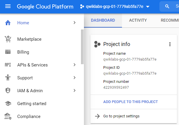
First, we need to go to `Console` by clicking the right upper corner button of the home page of https://cloud.google.com/.

Second, Google Cloud Console will help you to create a new project. It may take a few seconds to start this project. You will be able to view the `Project name` under the `Project Info` section after creating it.
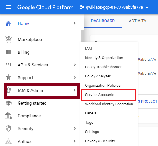
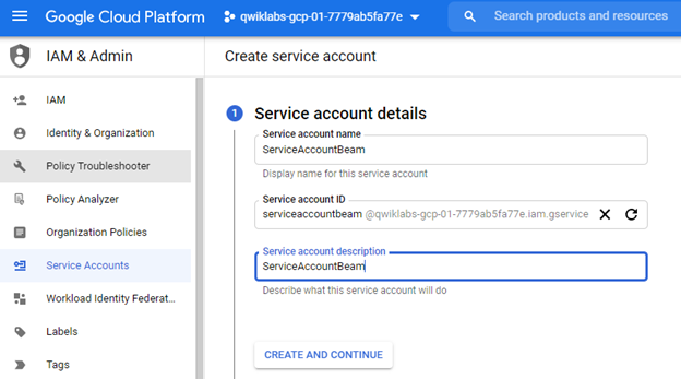
To get its `service_authentication_key`, we need to go to Service accounts which are found under the `IAM & Admin` section.
After we fill out the required fields, we can click on `Create and Continue`.
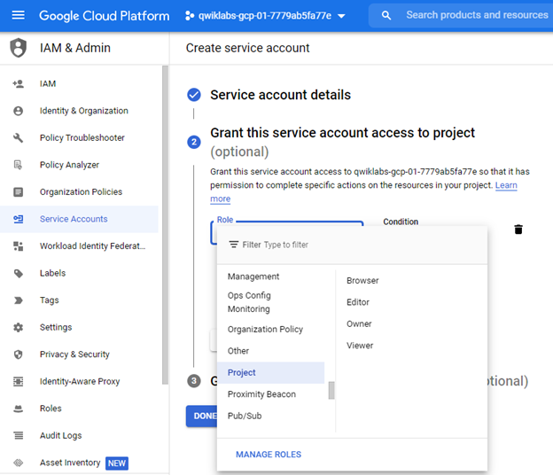
Optionally, you can grant the privileges you want in this authentication key. From the options, continue with `Project > Editor`.
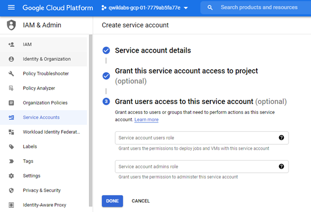
You can complete the initialization part by clicking the `DONE` button.
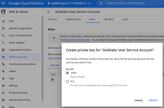
To create a `.json` formatted key, you can click on the `KEYS` tab and select `Create new key` under `ADD KEY`.
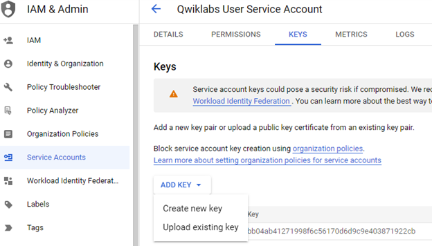
It is the key that we would like to generate for the service account. Download it and keep it in a very safe location. Anyone having this key can view your project.
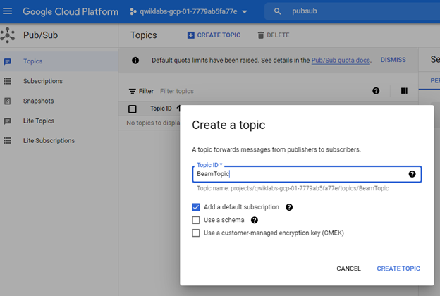
You will need a publisher, a topic, and a subscription. The publisher will publish the messages on a topic. To serve this purpose, we will be using `PubSub`.
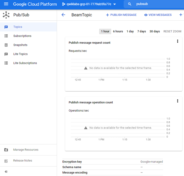
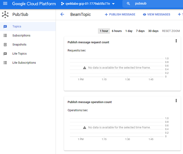
We have created the topic. Some of the statistics are `Publish message request count`, and `Published message operation count`. We are going to use this topic path in our publisher script.
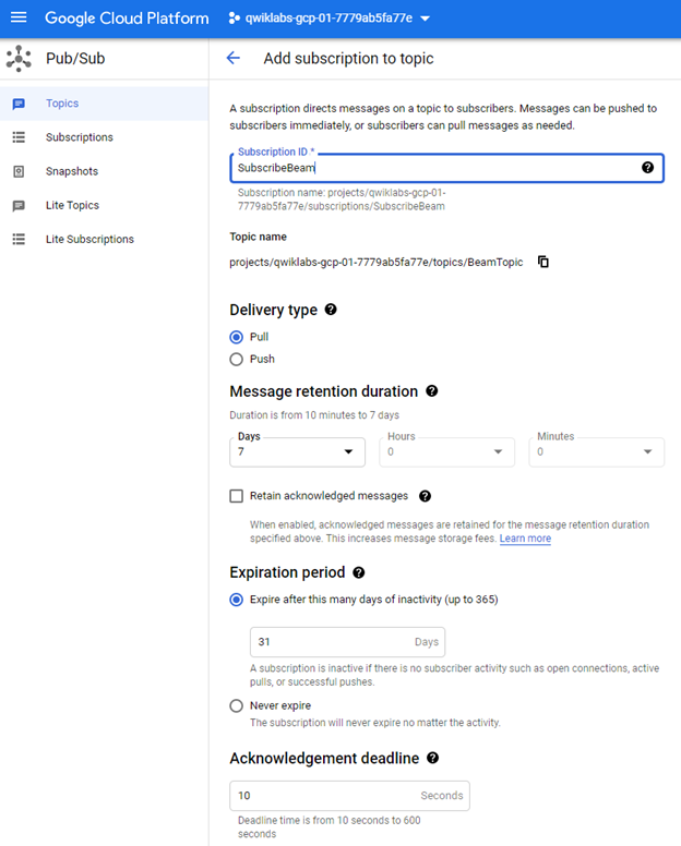
You need to create a subscription topic by filling in the subscription name and the `Delivery Type` as `Pull`.
After the topic and subscription are created, we can view statistics graphs that show nothing since we have not published any message yet.
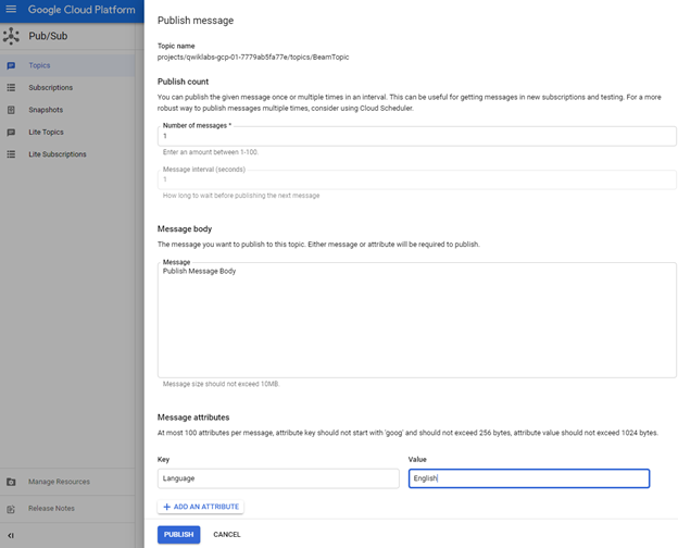
Suppose you wish to publish a message by using the interface itself. You can click on `Publish message` and provide optional message attributes as key-value pairs. These attributes are used to send additional information about the message. For `Add An Attributes`, you may add `Language` as key and `English` as its value.
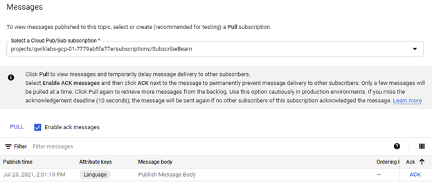
The message is published, and we can manually pull this message since there is no running subscriber. You may select the subscription through which you want to `PULL` it. You can check the enable acknowledgment button to send acknowledgment after receipt of it.
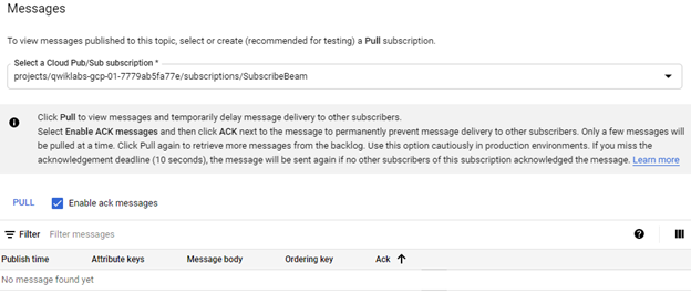
Then, you can click on `PULL`. You will view the message in addition to its attributes. We can observe that this message is acknowledged.
Some connectors are included in this whole activity to connect the client’s provider to our Publisher application. This approach follows in a few real-world scenarios, where rather than performing batch processing of the file, they want us to read the file line by line and have it processed.
The created PubSub topic can be defined in the script like the following to use it. You may replace the quoted strings with your specific paths. These paths should be filled to publish messages on the correct topic as mentioned in Google Cloud’s guide page [28].
import os
 from google.cloud import pubsub_v1

 project = ‘SubscribeBeam’

 topic_for_pubsub = ‘projects/qwiklabs-gcp-01–7779ab5fa77e/topics/BeamTopic’

 service_account_path = “C:\\Users\ersoyp\Documents\ApacheBeam\qwiklabs-gcp-01–7779ab5fa77e-2d40f7ded2a8.json”
 os.environ[“GOOGLE_APPLICATION_CREDENTIALS”] = service_account_path

 data_path = “C:\\Users\ersoyp\Documents\ApacheBeam\data.csv”
Processing Data Pipelines with GCP
In the previous section, we defined the PubSub topic and the related `service_account_path` information. For the following step, we will use the PubSub credentials to read and write data with Beam. Let’s implement it together.
The below script defined the PubSub topic path, service account path, input, and output file paths. Additionally, we added `GOOGLE_APPLICATION_CREDENTIALS` as an environment variable. After assigning those paths, we initialized the Beam pipeline that we will work on. With the help of input and output paths, we easily read from the Google Cloud PubSub and then write back to our results to it.
import osimport os
import apache_beam as beam
from apache_beam.options.pipeline_options import PipelineOptions, StandardOptions
from apache_beam import window
project = ‘SubscribeBeam’

pubsub_topic = ‘projects/qwiklabs-gcp-01–7779ab5fa77e/topics/BeamTopic’

path_service_account = “C:\\Users\ersoyp\Documents\ApacheBeam\qwiklabs-gcp-01–7779ab5fa77e-2d40f7ded2a8.json”

os.environ[“GOOGLE_APPLICATION_CREDENTIALS”] = path_service_account

input_file = “C:\\Users\ersoyp\Documents\ApacheBeam\data.csv”

output_file = ‘C:\\Users\ersoyp\Documents\ApacheBeam\output.csv’

options = PipelineOptions()

options.view_as(StandardOptions).streaming = True

process = beam.Pipeline(options=options)

output_file = ‘/content/outputs/’

pubsub_data = ( process
 |’Read from Google PubSub’ >> beam.io.ReadFromPubSub(subscription= input_file)
 |’Write to Google PubSub’ >> beam.io.WriteToPubSub(output_file))

final_file = process.run()
Subscribing Data Pipelines with GCP
As the final step for deploying data pipelines, we need to create a `SubscriberClient` object with PubSub. After the initialization of the subscriber, it will be assigned to the corresponding subscription path. You may view the implementation with the below script.
The script starts with assigning the `GOOGLE_APPLICATION_CREDENTIALS` as an environment variable in the operating system. The assigned path includes the service account key that is generated from the GCP IAM & Admin interface. After that, we create a path for subscription with the help of `args`. Then we create a SubcriberClient with GCP PubSub. At last, we assign the subscription path that we constructed to the GCP PubSub subscribers.
from google.cloud import pubsub_v1
import time
import os

os.environ[“GOOGLE_APPLICATION_CREDENTIALS”] = ‘C:\\Users\ersoyp\Documents\ApacheBeam\qwiklabs-gcp-01–7779ab5fa77e-2d40f7ded2a8.json’

path_for_subcription = args.subscription_path

pubsub_subscriber = pubsub_v1.SubscriberClient()

pubsub_subscriber.subscribe(path_for_subcription, callback=callback)
Monitoring Data Pipelines
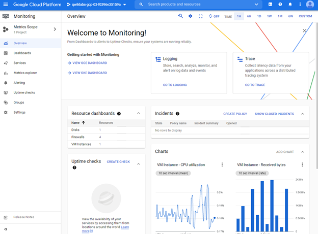
We published, processed, and subscribed the data pipelines with sample scripts with the help of Google Cloud PubSub in the above sections. Since we used GCP, we can follow the monitoring activities using the Google Cloud Monitoring tool.
With this aim, we can select Monitoring to view the `Overview`, `Dashboard`, `Services`, `Metrics explorer` by using this pane.
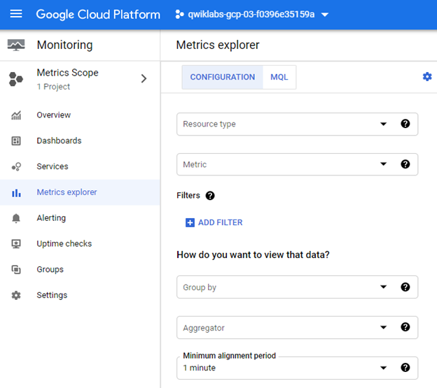
Any metric that we create will be added under the `Metrics explorer` tab. We may select `Resource type` and `Metric` to filter out the correct data. In addition, we can use the aggregation operations of `Group by` and `Aggregator` with an `Alignment period`.
Apache Beam vs. Apache Spark
Apache Beam produces pipelines in various environments. It is just another programming model for distributed data [28]. As in Apache Spark, Apache Beam has RDD’s or data frames to perform batch processing and data streams for stream processing. The Beam is implemented in Java, Python, and Go languages.
On the other hand, Apache Spark is a comprehensive engine for massive data processing. It was being developed in 2012 and initially designed for batch processing only. Spark breaks the stream into several small batches and processes these micro-batches.
If we keep the small batch size, it will seem as if we are performing real-time streaming data. That is why Spark is considered near to a real-time stream processing engine and not a valid stream processing engine. Spark is implemented in Scala language. It is also compatible with the Hadoop platform as described in Spark’s official page [29].
Final Thoughts
Throughout this article, a wide range of subjects are presented in the structure of initially describing the concept and implementing the solutions with sample scripts. The topics contain introducing Apache Beam, followed by building pipelines in Beam. The headings involved but are not limited to:
- The Architecture of Apache Beam
- The Features of Apache Beam
- The Pipeline Structure of Apache Beam
- ParDo Transformations
- Composite Transformations
- Side Inputs and Side Outputs
- Implementing Windows in Apache Beam
- Encoding Operation with Coder
- Apache Beam Triggers
- Structure of Streaming Data Pipeline
- Deploying Data Pipelines
- Monitoring Data Pipelines
- Apache Beam vs. Apache Spark
Questions and comments are highly appreciated!
Additional References
- Apache Beam: https://beam.apache.org/documentation/
- Apache Beam Pipeline: https://beam.apache.org/documentation/pipelines/design-your-pipeline/
- Apache Spark: https://spark.apache.org/documentation.html, https://beam.apache.org/documentation/runners/spark/
- Apache Flink: https://ci.apache.org/projects/flink/flink-docs-master/
- Apache Samza: http://samza.apache.org/startup/quick-start/1.6.0/beam.html
- Google Cloud Dataflow: https://cloud.google.com/dataflow/docs/concepts/beam-programming-model
- Big Data Description: https://www.sas.com/en_us/insights/big-data/what-is-big-data.html
- Apache Beam | A Hands-On course to build Big data Pipelines: https://www.udemy.com/course/apache-beam-a-hands-on-course-to-build-big-data-pipelines/
- The Window Accumulation Mode, https://beam.apache.org/documentation/programming-guide/#triggers
- Google Cloud Console, https://console.cloud.google.com
Data Pipelines with Apache Beam was originally published in Towards Data Science on Medium, where people are continuing the conversation by highlighting and responding to this story.
from Towards Data Science - Medium https://ift.tt/3pnYNWH
via RiYo Analytics


No comments