https://ift.tt/2ZG79OE We can create new deep neural networks by changing very few lines of code of already proposed models. Image by aut...
We can create new deep neural networks by changing very few lines of code of already proposed models.
When dealing with supervised learning within deep learning, we might say that there are some classical approaches to follow. The first solution is the so-called “heroic” strategy where one creates a completely new deep neural network (DNN) from scratch and train/evaluate it. In practical terms, this solution may not be very interesting since there are countless DNNs available nowadays, like many deep convolutional neural networks (CNNs), that can be reused. The second path is simply to consider a deployable DNN, trained for a certain context, and see its operation in another context. Despite all the advances in deep learning, models can present bad performances if the contexts are too diverse.
One of the most famous approach today is known as transfer learning which is used to improve a model from one domain (context) by transferring information from a related domain. The motivation to rely on transfer learning is when we face the situation where there are not so many samples in the training dataset. Some reasons for this are that the data are not cheap to collect and label or they are rare.

But, transfer learning may have disadvantages. Usually the models are trained on huge datasets so that such pretrained models can be reused in another context. Hence, we start the training not from scratch but based on an acquired “intelligence” embedded in the pretrained models. However, even if we have great number of images to train, the training dataset must be general enough to address different contexts. There are many interesting benchmark image sets such as ImageNet and COCO that aim to address this issue. But, eventually, we may be working in a challenging domain (e.g. autonomous driving, remote sensing) where transfer learning based on these classical datasets might not be enough.
Even if we have many attempts to augment the training samples, e.g. data augmentation, generative adversarial networks (GANs), we can create new models by reusing and/or making some modifications and/or combining different characteristics of other already proposed models. One of the most significant examples of such a strategy are the famous object detection DNNs called YOLO. These models, particularly version 4, were developed based on dozens of other solutions. Such networks are a kind of eclectic mixture of different concepts to obtain a new model, and they have been very successful for detecting objects in images and videos. Note that YOLOX is the newest version of the YOLO networks.
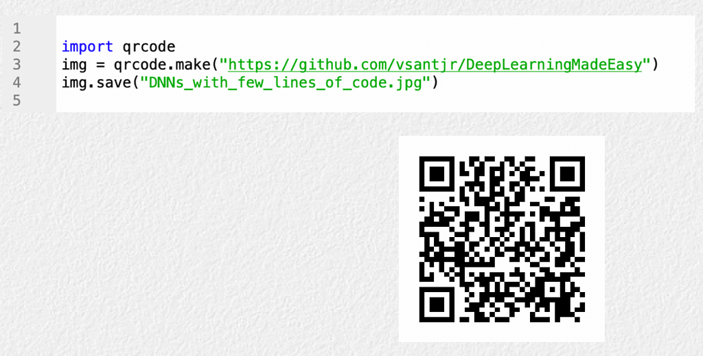
This post is in the direction to create new models by accomplishing a few variations in previously proposed approaches. It shows how easy it can be to create “new” DNNs by changing very few lines of code of previously proposed models. Note that we are pushing it a little by calling the networks presented below as “new” since the changes we have done were basically related to the number of layers of the original models. But, the whole point is to encourage practitioners to think about this, and eventually reuse/adapt previous ideas to generate new approaches when using DNNs in their practical settings.
VGG12BN
Top position in localisation and second best place in the classification task in the 2014 ImageNet Large Scale Visual Recognition Challenge (ILSVRC), VGG is one classical DNN which still has some uses today, even if some authors consider it an obsolete network. In the original article, authors proposed VGGs with 11, 13, 16, and 19 layers. Here, we show how to create a “new” VGG composing of 12 layers and with batch normalisation (BN) just by adding/changing 5 lines of code: VGG12BN.
We relied on the implementation of the PyTorch Team and modified it to create our model. The VGG modified code is here and the notebook to use it is here. Moreover, we considered a slightly modified version of the imagenette 320 px dataset from fastai. The difference is that the original validation dataset was split into two: validation dataset with 1/3 of the images of the original validation set, and 2/3 of the images compose the test dataset. Hence, there are 9,469 images (70.7%) in the training, 1,309 images (9.78%) in the validation, and 2,616 images (19.53%) in the test sets. It is a multiclass classification problem with 10 classes. We called the dataset as imagenettetvt320.
We now show the modifications we made in the VGG implementation of the PyTorch Team:
- Firstly, we commented out from .._internally_replaced_utils import load_state_dict_from_urlto avoid dependencies on other PyTorch modules. Also, to be completely sure that we will not use the pretrained models (by default pretrained = False), we commented outmodel_urls. It is just to emphasise this point and it is not really necessary to do this;
- The first modification is the addition of the name of our model: "vgg12_bn”;

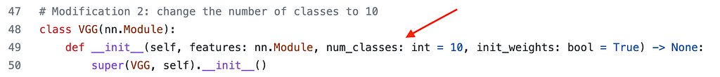
- Since we have 10 classes, we changed num_classes from 1000 to 10;
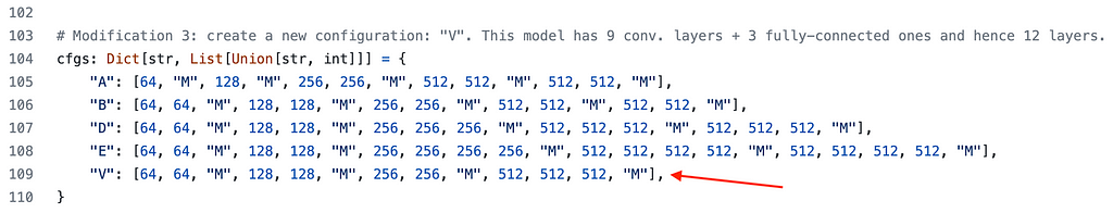
- Hence, we create a new configuration, "V", with the following convolutional layers (number of channels of each layer is shown in the sequence): 64, 64, 128, 128, 256, 256, 512, 512, 512. Note that "M" below means max pooling. Since VGG has 3 fully-connected (FC) layers by default, altogether we have 12 layers;
- To conclude, we create a function, vgg12_bn, which has just one line of code calling another function. Note that we see the values of parameters "vgg12_bn"(the name of the network), "V"(the configuration), and True where the latter activates batch normalisation.
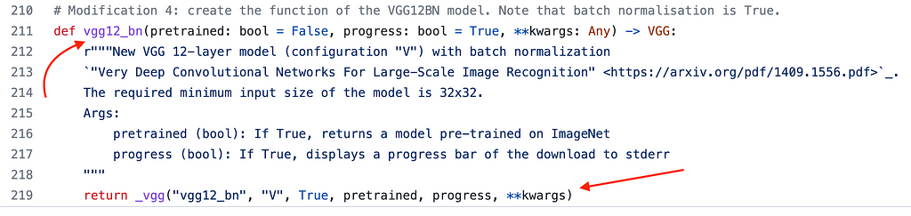
That is it. With 5 added/modified lines of code we created our model. In the notebook, we need to import the vggmodifiedfile to use the VGG12BN.
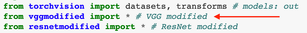
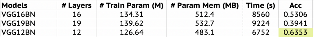
Figure (table) below shows the results in terms of accuracy (Acc) based on the test dataset after the training for 10 epochs. We compared the original VGG16BN, VGG19BN and the proposed VGG12BN models. Columns # Train Param (M), # Param Mem (MB), Time (s) present the number of million of trainable parameters of each model, the size in MByte only due to the parameters of the model, and the time to execute them using Google Colab. Our “new” VGG12BN got the higher accuracy.
DenseNet-83 and ResNet-14
In the DenseNet model, each layer is connected to every other layer in a feed-forward manner aiming to maximise the information flow between layers. Another winner of the ILSVRC, in 2015, ResNet is one of the most popular CNNs where several variants of it have already been proposed (ResNeXt, Wide ResNet, …) and it has also been reused as part of other DNNs. It is a residual learning approach where stacked layers fit a residual mapping rather than directly fitting a desired underlying mapping. We followed a similar procedure as we have just presented for VGG12BN, but now we had to change only 3 lines of code to create the DenseNet-83 (83 layers) and ResNet-14 (14 layers).
Access here the DenseNet modified code and its respective notebook is here. The ResNet modified code is here and the notebook is the same as the VGG12BN but now we show the output by running ResNet-14. Since the modifications to create both networks are similar, we will show below only the ones to create DenseNet-83. Hence, this is what we made:
- As previously, we commented out from .._internally_replaced_utils import load_state_dict_from_urlto avoid dependencies on other PyTorch modules. But note that we did not comment out models_urlnow;
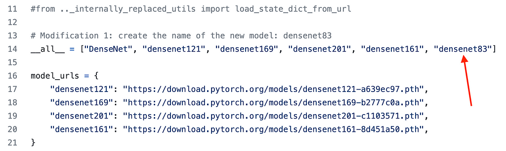
- We added the name of our model: "densenet83";
- And we create a function, densenet83, which has just one line of code calling another function. Note that we see the values of parameters "densenet83"(the name of the network), and (3, 6, 18, 12) are the number of repetitions of dense blocks 1, 2, 3, and 4, respectively.
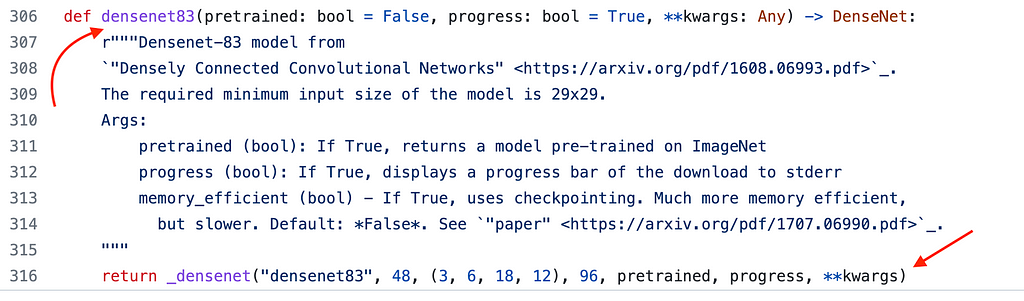
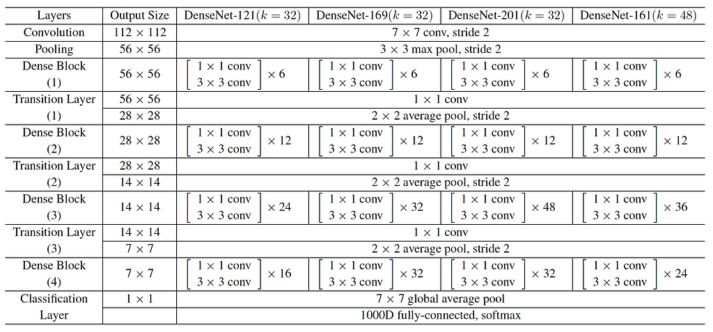
Figure below shows the DenseNet architectures for ImageNet. We considered DenseNet-161 as a reference and halved the number of repetitions of the blocks to derive the DenseNet-83.
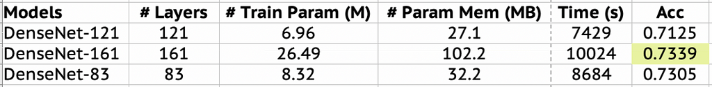
Altogether, 3 lines of code were added/modified. As for DenseNet, figure (table) below shows the results in terms of accuracy (Acc) based on the test dataset after the training for 10 epochs. We compared the original DenseNet-121, DenseNet-161 and the proposed DenseNet-83 models. We basically see a tie in terms of performance between DenseNet-161 and our “new” DenseNet-83, with DenseNet-161 being slightly superior.
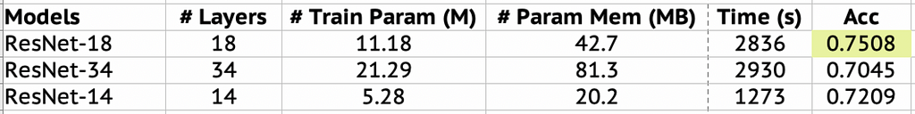
Regarding ResNet, comparing ResNet-18, ResNet-34, and the “new” ResNet-14, ResNet-18 was the best and ResNet-14 got the second place as shown in the figure (table) below.
Conclusions
In this post, we show how easy it can be to create new DNNs by modifying a few lines of code of previously proposed networks. We claim that reusing previous ideas and deriving new models with suitable modifications is a good path to follow.
Creating deep neural networks with 3 to 5 lines of code was originally published in Towards Data Science on Medium, where people are continuing the conversation by highlighting and responding to this story.
from Towards Data Science - Medium https://ift.tt/3bpV0Qm
via RiYo Analytics


ليست هناك تعليقات